
Those are my notes on taking some LiDAR data and testing different commands in PDAL. If you like, you can follow along using your own data.
Most probably I’ll de adding or deleting stuff, but you can take a look to see some of the main operations that can be made on point clouds using PDAL.
This is an adaptation of the original workshop from the PDAL website, Point Cloud Processing and Analysis with PDAL, the single difference being that I use the same data for every operation and show the commands output, too, while in the workshop there are used different data sources. Also, because the files were large, I had to make tiles and use batch processing for some operations.
The workshop can be downloaded from here, too.
The colored point cloud data that we will be using throughout this post can be viewed here: https://potree.entwine.io/data/view.html?r=”https://maptheclouds.com/ept_yose_colored/”.
You can use Fugro Viewer or LASTools to view LiDAR files on desktop, but only in Windows! The Linux users, although forgotten, are lucky to have Potree and Plasio that can consume Entwine Point Tile (EPT) datasets in the browser. But let’s just approach LiDAR with baby steps before digging too deep. 🙂
LiDAR refers to a remote sensing technology that emits intense, focused beams of light and measures the time it takes for the reflections to be detected by the sensor. This information is used to compute ranges, or distances, to objects. In this manner, lidar is analogous to radar (radio detecting and ranging), except that it is based on discrete pulses of laser light. The three-dimensional coordinates (e.g., x,y,z or latitude, longitude, and elevation) of the target objects are computed from 1) the time difference between the laser pulse being emitted and returned, 2) the angle at which the pulse was “fired,” and 3) the absolute location of the sensor on or above the surface of the Earth.

lidar
I won’t go into details about LiDAR, feel free to read this comprehensive guide: Lidar 101: An Introduction to Lidar Technology, Data, and Applications.
Download the data
You can use your own files, but I’ll be using free data for Yosemite Valley.
There are three point clouds of LAS type for Yosemite Valley on OpenTopography. In order to conduct this study in the area, the files were downloaded, merged and transformed into raster files. One file was too large, it was splitted in two for download, resulting four files for processing. We will convert the files to LAZ format, too, in order to save space.
The original files and the job ids used to download and split the data are:
- Yosemite National Park, CA: Rockfall Studies. Distributed by OpenTopography. https://doi.org/10.5069/G9D798B8. Accessed: 2019-12-10
- Yosemite, CA: El Portal, Mariposa Grove, Yosemite Canyon & Tuolumne Meadows. Distributed by OpenTopography. https://doi.org/10.5069/G9GQ6VP3. Accessed: 2019-12-10
- Airborne Laser Mapping of Yosemite National Park, CA, 2007. Distributed by OpenTopography. https://doi.org/10.5069/G9W66HPH. Accessed: 2019-12-10
raw_data/
├── points_extra_yose.las
├── points_little_yose.las
├── points_rockfall_1.las
└── points_rockfall_2.las
rockfall 1 
rockfall 2 
little yosemite 
extended yosemite
We create a working folder, yose and a subfolder named raw_data, then move all the downloaded point cloud data into it.
# go home, create subdirectory and parent directory
cd && mkdir -pv yose/raw_data
Install PDAL
You can read this other post to find out how to install PDAL. Every time you want to access the environment where PDAL was installed, useconda activate followed by the environment name, in our case new_clouds.
I will refer to Linux, though the commands for Windows will be mentioned, too. NOTE: PDAL commands, except batch processing, are the same in Windows and Linux, but the line separator differs: ^ in Windows and \ in Linux.
Play
Printing the first point (src)
# List the LAZ files
cd ~/yose
ls -lah raw_data
# Query the las data using pdal info
pdal info raw_data/points_little_yose.las -p 0
pdal info raw_data/points_extra_yose.las -p 0
pdal info raw_data/points_rockfall_1.las -p 0
(new_clouds) myuser@comp:~/yose$ pdal info raw_data/points_little_yose.las -p 0
{
"filename": "raw_data/points_little_yose.las",
"pdal_version": "2.0.1 (git-version: 6600e6)",
"points":
{
"point":
{
"Blue": 0,
"Classification": 1,
"EdgeOfFlightLine": 0,
"GpsTime": 397906.1493,
"Green": 0,
"Intensity": 0,
"NumberOfReturns": 1,
"PointId": 0,
"PointSourceId": 0,
"Red": 0,
"ReturnNumber": 1,
"ScanAngleRank": 28,
"ScanDirectionFlag": 0,
"UserData": 32,
"X": 278287.53,
"Y": 4179655.54,
"Z": 1986.66
}
}
}
(new_clouds) myuser@comp:~/yose$ pdal info raw_data/points_extra_yose.las -p 0
{
"filename": "raw_data/points_extra_yose.las",
"pdal_version": "2.0.1 (git-version: 6600e6)",
"points":
{
"point":
{
"Classification": 1,
"EdgeOfFlightLine": 0,
"Intensity": 0,
"NumberOfReturns": 1,
"PointId": 0,
"PointSourceId": 0,
"ReturnNumber": 1,
"ScanAngleRank": 0,
"ScanDirectionFlag": 0,
"UserData": 0,
"X": 266398.74,
"Y": 4180473.61,
"Z": 2261.31
}
}
}
(new_clouds) myuser@comp:~/yose$ pdal info raw_data/points_rockfall_1.las -p 0
{
"filename": "raw_data/points_rockfall_1.las",
"pdal_version": "2.0.1 (git-version: 6600e6)",
"points":
{
"point":
{
"Classification": 12,
"EdgeOfFlightLine": 0,
"GpsTime": 502909.1808,
"Intensity": 17,
"NumberOfReturns": 3,
"PointId": 0,
"PointSourceId": 3,
"ReturnNumber": 3,
"ScanAngleRank": -18,
"ScanDirectionFlag": 0,
"UserData": 32,
"X": 272126.59,
"Y": 4182001.04,
"Z": 1663.82
}
}
}
(new_clouds) myuser@comp:~/yose$Printing file metadata (src)
pdal info raw_data/points_little_yose.las --metadata(new_clouds) myuser@comp:~/yose$ pdal info raw_data/points_little_yose.las --metadata
{
"filename": "raw_data/points_little_yose.las",
"metadata":
{
"comp_spatialreference": "PROJCS[\"NAD83 / UTM zone 11N\",GEOGCS[\"NAD83\",DATUM[\"North_American_Datum_1983\",SPHEROID[\"GRS 1980\",6378137,298.257222101,AUTHORITY[\"EPSG\",\"7019\"]],TOWGS84[0,0,0,0,0,0,0],AUTHORITY[\"EPSG\",\"6269\"]],PRIMEM[\"Greenwich\",0,AUTHORITY[\"EPSG\",\"8901\"]],UNIT[\"degree\",0.0174532925199433,AUTHORITY[\"EPSG\",\"9122\"]],AUTHORITY[\"EPSG\",\"4269\"]],PROJECTION[\"Transverse_Mercator\"],PARAMETER[\"latitude_of_origin\",0],PARAMETER[\"central_meridian\",-117],PARAMETER[\"scale_factor\",0.9996],PARAMETER[\"false_easting\",500000],PARAMETER[\"false_northing\",0],UNIT[\"metre\",1,AUTHORITY[\"EPSG\",\"9001\"]],AXIS[\"Easting\",EAST],AXIS[\"Northing\",NORTH],AUTHORITY[\"EPSG\",\"26911\"]]",
"compressed": false,
"count": 24659714,
"creation_doy": 353,
"creation_year": 2019,
"dataformat_id": 3,
"dataoffset": 513,
"filesource_id": 0,
"global_encoding": 0,
"global_encoding_base64": "AAA=",
"header_size": 227,
"major_version": 1,
"maxx": 285218.04,
"maxy": 4181646.22,
"maxz": 2906.555,
"minor_version": 2,
"minx": 277177.53,
"miny": 4178720.94,
"minz": 1853.189,
"offset_x": 0,
"offset_y": 0,
"offset_z": 0,
"point_length": 34,
"project_id": "00000000-0000-0000-0000-000000000000",
"scale_x": 0.01,
"scale_y": 0.01,
"scale_z": 0.01,
"software_id": "PDAL 2.0.1 (Releas)",
"spatialreference": "PROJCS[\"NAD83 / UTM zone 11N\",GEOGCS[\"NAD83\",DATUM[\"North_American_Datum_1983\",SPHEROID[\"GRS 1980\",6378137,298.257222101,AUTHORITY[\"EPSG\",\"7019\"]],TOWGS84[0,0,0,0,0,0,0],AUTHORITY[\"EPSG\",\"6269\"]],PRIMEM[\"Greenwich\",0,AUTHORITY[\"EPSG\",\"8901\"]],UNIT[\"degree\",0.0174532925199433,AUTHORITY[\"EPSG\",\"9122\"]],AUTHORITY[\"EPSG\",\"4269\"]],PROJECTION[\"Transverse_Mercator\"],PARAMETER[\"latitude_of_origin\",0],PARAMETER[\"central_meridian\",-117],PARAMETER[\"scale_factor\",0.9996],PARAMETER[\"false_easting\",500000],PARAMETER[\"false_northing\",0],UNIT[\"metre\",1,AUTHORITY[\"EPSG\",\"9001\"]],AXIS[\"Easting\",EAST],AXIS[\"Northing\",NORTH],AUTHORITY[\"EPSG\",\"26911\"]]",
[...]
"units":
{
"horizontal": "metre",
"vertical": ""
},
"vertical": "",
"wkt": "PROJCS[\"NAD83 / UTM zone 11N\",GEOGCS[\"NAD83\",DATUM[\"North_American_Datum_1983\",SPHEROID[\"GRS 1980\",6378137,298.257222101,AUTHORITY[\"EPSG\",\"7019\"]],TOWGS84[0,0,0,0,0,0,0],AUTHORITY[\"EPSG\",\"6269\"]],PRIMEM[\"Greenwich\",0,AUTHORITY[\"EPSG\",\"8901\"]],UNIT[\"degree\",0.0174532925199433,AUTHORITY[\"EPSG\",\"9122\"]],AUTHORITY[\"EPSG\",\"4269\"]],PROJECTION[\"Transverse_Mercator\"],PARAMETER[\"latitude_of_origin\",0],PARAMETER[\"central_meridian\",-117],PARAMETER[\"scale_factor\",0.9996],PARAMETER[\"false_easting\",500000],PARAMETER[\"false_northing\",0],UNIT[\"metre\",1,AUTHORITY[\"EPSG\",\"9001\"]],AXIS[\"Easting\",EAST],AXIS[\"Northing\",NORTH],AUTHORITY[\"EPSG\",\"26911\"]]"
},
"system_id": "PDAL",
"vlr_0":
{
"data": "AQABAAAACAAABAAAAQABAAEEAAABAAEAAgSxhxUAAAABCLGHBgAVAAYIAAABAI4jDgiwhwMAAAAADAAAAQAfaQQMAAABACkj",
"description": "GeoTiff GeoKeyDirectoryTag",
"record_id": 34735,
"user_id": "LASF_Projection"
},
"vlr_1":
{
"data": "AAAAAAAAAAAAAAAAAAAAAAAAAAAAAAAA",
"description": "GeoTiff GeoDoubleParamsTag",
"record_id": 34736,
"user_id": "LASF_Projection"
},
"vlr_2":
{
"data": "TkFEODMgLyBVVE0gem9uZSAxMU58TkFEODN8AA==",
"description": "GeoTiff GeoAsciiParamsTag",
"record_id": 34737,
"user_id": "LASF_Projection"
}
},
"pdal_version": "2.0.1 (git-version: 6600e6)"
}
(new_clouds) myuser@comp:~/yose$Install jq with sudo apt install jq (on Windows from https://stedolan.github.io/jq), then filter the JSON query result using jq.
pdal info raw_data/points_little_yose.las --metadata | jq  ".metadata.maxx, .metadata.count"
pdal info raw_data/points_extra_yose.las --metadata | jq  ".metadata.maxx, .metadata.count"
pdal info raw_data/points_rockfall_1.las --metadata | jq  ".metadata.maxx, .metadata.count"
pdal info raw_data/points_rockfall_2.las --metadata | jq  ".metadata.maxx, .metadata.count"
(new_clouds) myuser@comp:~/yose$ pdal info raw_data/points_little_yose.las --metadata | jq ".metadata.maxx, .metadata.count"
285218.04
24659714
(new_clouds) myuser@comp:~/yose$ pdal info raw_data/points_extra_yose.las --metadata | jq ".metadata.maxx, .metadata.count"
279109.57
242928874
(new_clouds) myuser@comp:~/yose$ pdal info raw_data/points_rockfall_1.las --metadata | jq ".metadata.maxx, .metadata.count"
273832.49
137631935
(new_clouds) myuser@comp:~/yose$ pdal info raw_data/points_rockfall_2.las --metadata | jq ".metadata.maxx, .metadata.count"
279499.99
165274810
(new_clouds) myuser@comp:~/yose$Find the midpoint of the bounding cube (src)
(new_clouds) myuser@comp:~/yose$ pdal info raw_data/points_little_yose.las --all | jq .stats.bbox.native.bbox{
  "maxx": 285218.04,
  "maxy": 4181646.22,
  "maxz": 2906.56,
  "minx": 277177.53,
  "miny": 4178720.94,
  "minz": 1853.19
}
(new_clouds) myuser@comp:~/yose$
Calculate the average the X, Y, and Z values for this tile: min + (max – min)/2
- x = 277177.53 + (277177.53 – 277177.53)/2 = 277177.53
- y = 4178720.94 + (4181646.22 – 4178720.94)/2 = 4180183.58
- z = 1853.19 + (2906.56 – 1853.19)/2 = 2379.875
(new_clouds) myuser@comp:~/yose$ python
Python 3.8.1 | packaged by conda-forge | (default, Jan 29 2020, 14:55:04)
[GCC 7.3.0] on linux
Type "help", "copyright", "credits" or "license" for more information.
>>> 277177.53 + (277177.53 - 277177.53)/2
277177.53
>>> 4178720.94 + (4181646.22 - 4178720.94)/2
4180183.58
>>> 1853.19 + (2906.56 - 1853.19)/2
2379.875
>>> exit()
(new_clouds) myuser@comp:~/yose$
Now we can return the three nearest points from the calculated center (Note that we use /3).
pdal info raw_data/points_little_yose.las --query "277177.53, 4180183.58, 2379.875/3"(new_clouds) myuser@comp:~/yose$ pdal info raw_data/points_little_yose.las --query "277177.53, 4180183.58, 2379.875/3"
{
"filename": "raw_data/points_little_yose.las",
"pdal_version": "2.0.1 (git-version: 6600e6)",
"points":
{
"point":
[
{
"Blue": 0,
"Classification": 1,
"EdgeOfFlightLine": 0,
"GpsTime": 398668.7963,
"Green": 0,
"Intensity": 0,
"NumberOfReturns": 2,
"PointId": 15481196,
"PointSourceId": 0,
"Red": 0,
"ReturnNumber": 1,
"ScanAngleRank": 22,
"ScanDirectionFlag": 0,
"UserData": 32,
"X": 281470.21,
"Y": 4179214.96,
"Z": 2906.56
},
{
"Blue": 0,
"Classification": 1,
"EdgeOfFlightLine": 0,
"GpsTime": 398883.1897,
"Green": 0,
"Intensity": 41,
"NumberOfReturns": 1,
"PointId": 15647573,
"PointSourceId": 0,
"Red": 0,
"ReturnNumber": 1,
"ScanAngleRank": -8,
"ScanDirectionFlag": 0,
"UserData": 32,
"X": 280394.17,
"Y": 4181634.48,
"Z": 2632.03
},
{
"Blue": 0,
"Classification": 1,
"EdgeOfFlightLine": 0,
"GpsTime": 398883.1897,
"Green": 0,
"Intensity": 35,
"NumberOfReturns": 1,
"PointId": 15647574,
"PointSourceId": 0,
"Red": 0,
"ReturnNumber": 1,
"ScanAngleRank": -8,
"ScanDirectionFlag": 0,
"UserData": 32,
"X": 280394.77,
"Y": 4181634.46,
"Z": 2631.94
}
]
}
}
(new_clouds) myuser@comp:~/yose$Compression and Decompression (src)
Create a new folder named temp_data, decompress the file from LAZ to LAS or vice-versa using pdal translate, then compare their size. Note that it would take some time to complete the transformation, if the files were large, but after the compression the storage decreases significantly.
mkdir temp_data && pdal translate raw_data/points_little_yose.las temp_data/points_little_yose.laz
pdal translate raw_data/points_extra_yose.las temp_data/points_extra_yose.laz
pdal translate raw_data/points_rockfall_1.las temp_data/points_rockfall_1.laz
pdal translate raw_data/points_rockfall_2.las temp_data/points_rockfall_2.laz
ls -lah raw_data/points_little_yose.*
ls -lah raw_data/points_extra_yose.*
ls -lah raw_data/points_rockfall_1.*
ls -lah temp_data/points_rockfall_2.*
(new_clouds) myuser@comp:~/yose$ pdal translate raw_data/points_little_yose.las raw_data/points_little_yose.laz
(new_clouds) myuser@comp:~/yose$ pdal translate raw_data/points_extra_yose.las raw_data/points_extra_yose.laz
(new_clouds) myuser@comp:~/yose$ pdal translate raw_data/points_rockfall_1.las raw_data/points_rockfall_1.laz
(new_clouds) myuser@comp:~/yose$ pdal translate raw_data/points_rockfall_2.las raw_data/points_rockfall_2.laz
(new_clouds) myuser@comp:~/yose$ ls -lah raw_data/points_little_yose.*
-rwxrwxrwx 1 myuser myuser 800M dec 20 22:33 raw_data/points_little_yose.las
-rw-r--r-- 1 myuser myuser 78M feb 16 22:41 raw_data/points_little_yose.laz
(new_clouds) myuser@comp:~/yose$ ls -lah raw_data/points_extra_yose.*
-rwxrwxrwx 1 myuser myuser 4,6G dec 20 11:25 raw_data/points_extra_yose.las
-rw-r--r-- 1 myuser myuser 643M feb 16 22:43 raw_data/points_extra_yose.laz
(new_clouds) myuser@comp:~/yose$ ls -lah raw_data/points_rockfall_1.*
-rwxrwxrwx 1 myuser myuser 3,6G nov 29 17:54 raw_data/points_rockfall_1.las
-rw-r--r-- 1 myuser myuser 613M feb 16 22:44 raw_data/points_rockfall_1.laz
(new_clouds) myuser@comp:~/yose$ ls -lah raw_data/points_rockfall_2.*
-rwxrwxrwx 1 myuser myuser 4,4G nov 29 19:28 raw_data/points_rockfall_2.las
-rw-r--r-- 1 myuser myuser 708M feb 16 22:46 raw_data/points_rockfall_2.laz
(new_clouds) myuser@comp:~/yose$From now on we will use the compressed files in our operations.
Reprojection (src)
Reproject file using pdal translate to “EPSG:4326” for testing purposes.
pdal translate raw_data/points_little_yose.laz \
    temp_data/points_little_yose_wgs84.laz reprojection \
    --filters.reprojection.in_srs="EPSG:32611" \
    --filters.reprojection.out_srs="EPSG:4326"
pdal info temp_data/points_little_yose_wgs84.laz --all | jq .stats.bbox.native.bbox
pdal info temp_data/points_little_yose_wgs84.laz -p 0
(new_clouds) myuser@comp:~/yose$ pdal translate raw_data/points_little_yose.laz \
> temp_data/points_little_yose_wgs84.laz reprojection \
> --filters.reprojection.in_srs="EPSG:32611" \
> --filters.reprojection.out_srs="EPSG:4326"
(new_clouds) myuser@comp:~/yose$ pdal info temp_data/points_little_yose_wgs84.laz --all | jq .stats.bbox.native.bbox
{
"maxx": -119.44,
"maxy": 37.76,
"maxz": 2906.56,
"minx": -119.53,
"miny": 37.73,
"minz": 1853.19
}
(new_clouds) myuser@comp:~/yose$ pdal info temp_data/points_little_yose_wgs84.laz -p 0
{
"filename": "temp_data/points_little_yose_wgs84.laz",
"pdal_version": "2.0.1 (git-version: 6600e6)",
"points":
{
"point":
{
"Blue": 0,
"Classification": 1,
"EdgeOfFlightLine": 0,
"GpsTime": 397906.1493,
"Green": 0,
"Intensity": 0,
"NumberOfReturns": 1,
"PointId": 0,
"PointSourceId": 0,
"Red": 0,
"ReturnNumber": 1,
"ScanAngleRank": 28,
"ScanDirectionFlag": 0,
"UserData": 32,
"X": -119.52,
"Y": 37.74,
"Z": 1986.66
}
}
}
(new_clouds) myuser@comp:~/yose$
(new_clouds) myuser@comp:~/yose$For latitude/longitude data, you will need to set the scale to smaller values like 0.0000001. Repeat the reproject command setting the scale, too.
pdal translate raw_data/points_little_yose.las \
    temp_data/points_little_yose_wgs84.laz reprojection \
    --filters.reprojection.in_srs="EPSG:32611" \
    --filters.reprojection.out_srs="EPSG:4326" \
    --writers.las.scale_x=0.0000001 \
    --writers.las.scale_y=0.0000001 \
    --writers.las.offset_x="auto" \
    --writers.las.offset_y="auto"
pdal info temp_data/points_little_yose_wgs84.laz --all | jq .stats.bbox.native.bbox
pdal info temp_data/points_little_yose_wgs84.laz -p 0
(new_clouds) myuser@comp:~/yose$ pdal translate raw_data/points_little_yose.las \
> temp_data/points_little_yose_wgs84.laz reprojection \
> --filters.reprojection.in_srs="EPSG:32611" \
> --filters.reprojection.out_srs="EPSG:4326" \
> --writers.las.scale_x=0.0000001 \
> --writers.las.scale_y=0.0000001 \
> --writers.las.offset_x="auto" \
> --writers.las.offset_y="auto"
(pdal translate writers.las Warning) Auto offset for Xrequested in stream mode. Using value of -119.516.
(pdal translate writers.las Warning) Auto offset for Yrequested in stream mode. Using value of 37.7374.
(new_clouds) myuser@comp:~/yose$ pdal info temp_data/points_little_yose_wgs84.laz --all | jq .stats.bbox.native.bbox
{
"maxx": -119.4378776,
"maxy": 37.75570403,
"maxz": 2906.56,
"minx": -119.5286917,
"miny": 37.72952363,
"minz": 1853.19
}
(new_clouds) myuser@comp:~/yose$ pdal info temp_data/points_little_yose_wgs84.laz -p 0Entwine (src)
We will use Entwine to create a new folder named ept_yose, then rearrange points into a lossless octree structure known as EPT.
You can read this other post to find out how to install Entwine.
The build command is used to generate an Entwine Point Tile (EPT) dataset from point cloud data. Because we want to build the visualization from all of our data, for input we provide the path to raw_data folder the command. Note that we select only the LAZ files.
entwine build -i raw_data/*.laz -o ept_yose --srs "EPSG:26911"(new_clouds) myuser@comp:~/yose$ entwine build -i raw_data/*.laz -o ept_yose --srs "EPSG:26911"
Scanning input
1/4: raw_data/points_extra_yose.laz
2/4: raw_data/points_little_yose.laz
3/4: raw_data/points_rockfall_1.laz
4/4: raw_data/points_rockfall_2.laz
Entwine Version: 2.1.0
EPT Version: 1.0.0
Input:
Files: 4
Total points: 570,495,333
Density estimate (per square unit): 2.14675
Threads: [3, 5]
Output:
Path: ept_yose/
Data type: laszip
Hierarchy type: json
Sleep count: 2,097,152
Scale: 0.01
Offset: (273845, 4179692, 1924)
Metadata:
SRS: EPSG:26911
Bounds: [(262472, 4174883, 747), (285219, 4184500, 3101)]
Cube: [(262471, 4168317, -9451), (285221, 4191067, 13299)]
Storing dimensions: [
X:int32, Y:int32, Z:int32, Intensity:uint16, ReturnNumber:uint8,
NumberOfReturns:uint8, ScanDirectionFlag:uint8,
EdgeOfFlightLine:uint8, Classification:uint8, ScanAngleRank:float,
UserData:uint8, PointSourceId:uint16, GpsTime:double, Red:uint16,
Green:uint16, Blue:uint16, OriginId:uint32
]
Build parameters:
Span: 128
Resolution 2D: 128 * 128 = 16,384
Resolution 3D: 128 * 128 * 128 = 2,097,152
Maximum node size: 65,536
Minimum node size: 16,384
Cache size: 64
Adding 0 - raw_data/points_extra_yose.laz
Adding 1 - raw_data/points_little_yose.laz
Adding 2 - raw_data/points_rockfall_1.laz
Adding 3 - raw_data/points_rockfall_2.laz
Pushes complete - joining...
00:10 - 3% - 16,805,888 - 6,050(6,050)M/h - 47W - 0R - 411A
00:20 - 5% - 30,949,376 - 5,570(5,091)M/h - 345W - 64R - 453A
00:30 - 8% - 44,695,552 - 5,363(4,948)M/h - 339W - 42R - 502A
00:40 - 10% - 55,943,168 - 5,034(4,049)M/h - 410W - 105R - 461A
00:50 - 12% - 68,812,800 - 4,954(4,633)M/h - 438W - 70R - 429A
01:00 - 14% - 79,781,888 - 4,786(3,948)M/h - 297W - 160R - 565A
Done 1
01:10 - 16% - 89,364,226 - 4,595(3,449)M/h - 432W - 105R - 437A
01:20 - 18% - 100,562,690 - 4,525(4,031)M/h - 241W - 80R - 537A
[...]
18:40 - 98% - 561,742,971 - 1,805(470)M/h - 662W - 11R - 288A
18:50 - 99% - 564,921,467 - 1,799(1,144)M/h - 108W - 61R - 298A
19:00 - 100% - 569,181,307 - 1,797(1,533)M/h - 96W - 22R - 313A
19:10 - 100% - 570,495,333 - 1,785(473)M/h - 284W - 91R - 157A
Done 0
Reawakened: 14846
Saving registry...
Saving metadata...
Index completed in 19:12.
Save complete.
Points inserted: 570,495,333
(new_clouds) myuser@comp:~/yose(new_clouds) myuser@comp:~/yose$ tree ept_yose/
ept_yose/
├── ept-build.json
├── ept-data
│ ├── 0-0-0-0.laz
│ ├── 1-0-0-0.laz
│ ├── 1-0-0-1.laz
[...]
│ ├── 9-314-267-269.laz
│ ├── 9-314-281-255.laz
│ └── 9-314-326-252.laz
├── ept-hierarchy
│ └── 0-0-0-0.json
├── ept.json
└── ept-sources
├── 0.json
└── list.json
3 directories, 12972 files
(new_clouds) myuser@comp:~/yose$Now we can statically serve the entwine directory with an HTTP server and visualize it with the WebGL-based Potree and Plasio projects.
Potree and Plasio
We can visualize our data in Potree and Plasio, directly in the browser.
# Install NodeJS and http server from nodejs
conda install nodejs -y
npm install http-server -g
# Make sure you are in the working folder, and the EPT folder
# is a subfolder
# Start the server using --cors to allow serving data to the
# remote Potree/Plasio pages
http-server -p 8066 --cors
(new_clouds) myuser@comp:~/yose$ http-server -p 8066 --cors
Starting up http-server, serving ./
Available on:
http://127.0.0.1:8066
http://192.168.0.102:8066
http://172.18.0.1:8066
http://192.168.61.1:8066
http://192.168.63.1:8066
Hit CTRL-C to stop the server# In another tab (Shift+Ctrl+T), visualise out local point cloud data in Potree
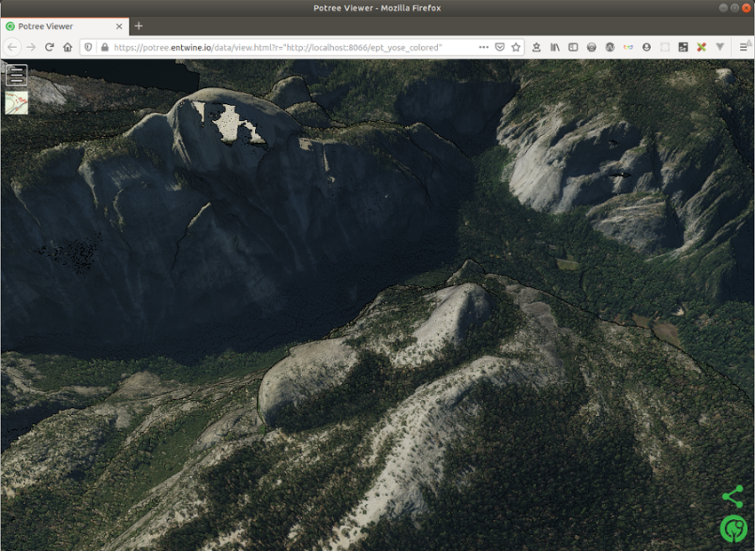
xdg-open "http://potree.entwine.io/data/view.html?r=http://localhost:8066/ept_yose"Assign a colour scale to the points based on elevation, classification and other criteria, then play with some terrain profiles.

first view 
elevation 
el capitan profile 
inner profile 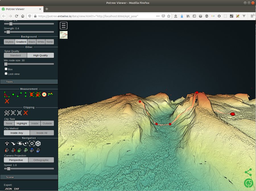
the dome profile 
inner profile 
elevation 
ground only 
ground & unclassified 
about
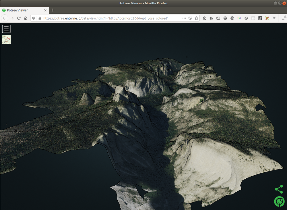
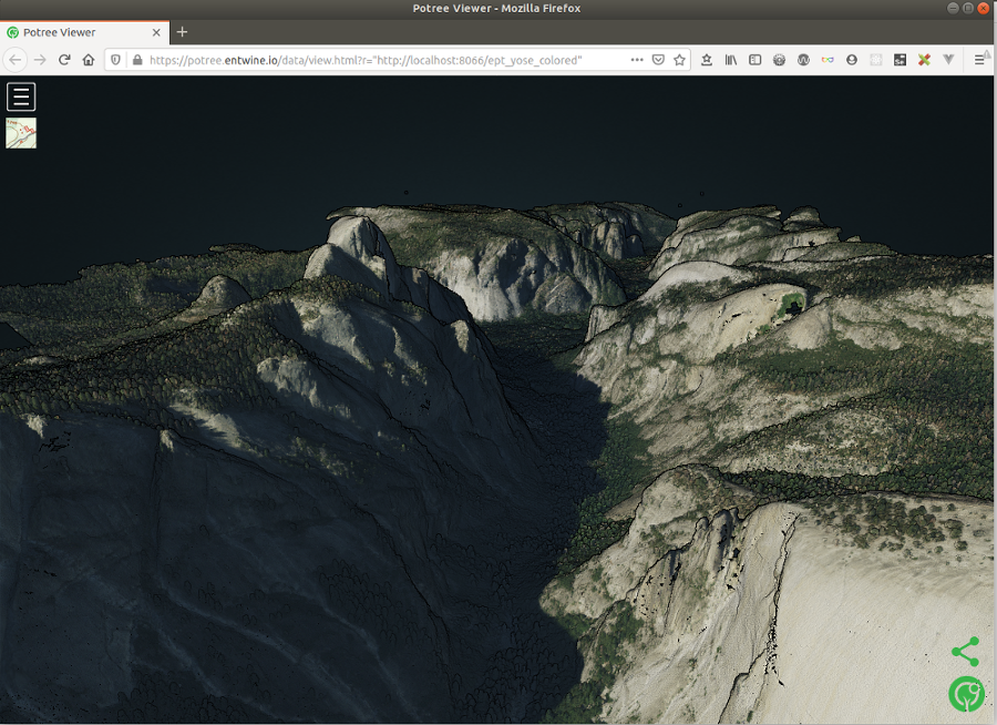
Visualize the points by elevation:
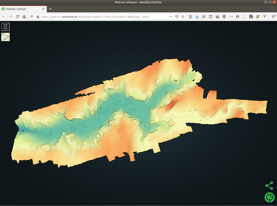
top view 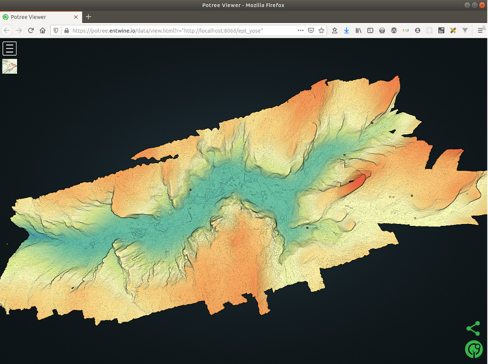
top zoom 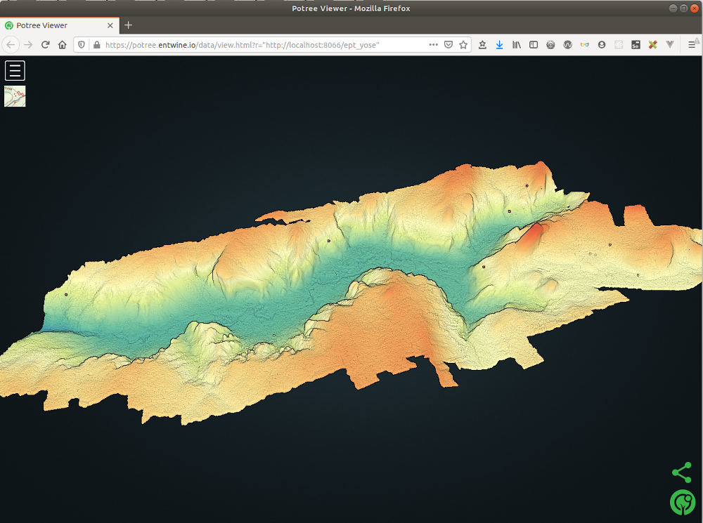
front view 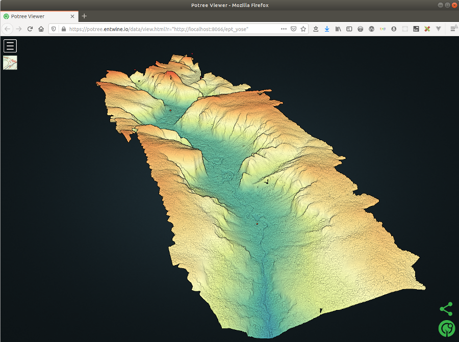
left view 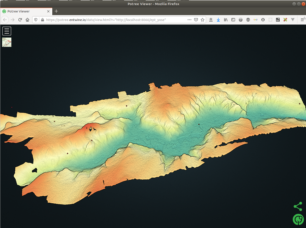
back view 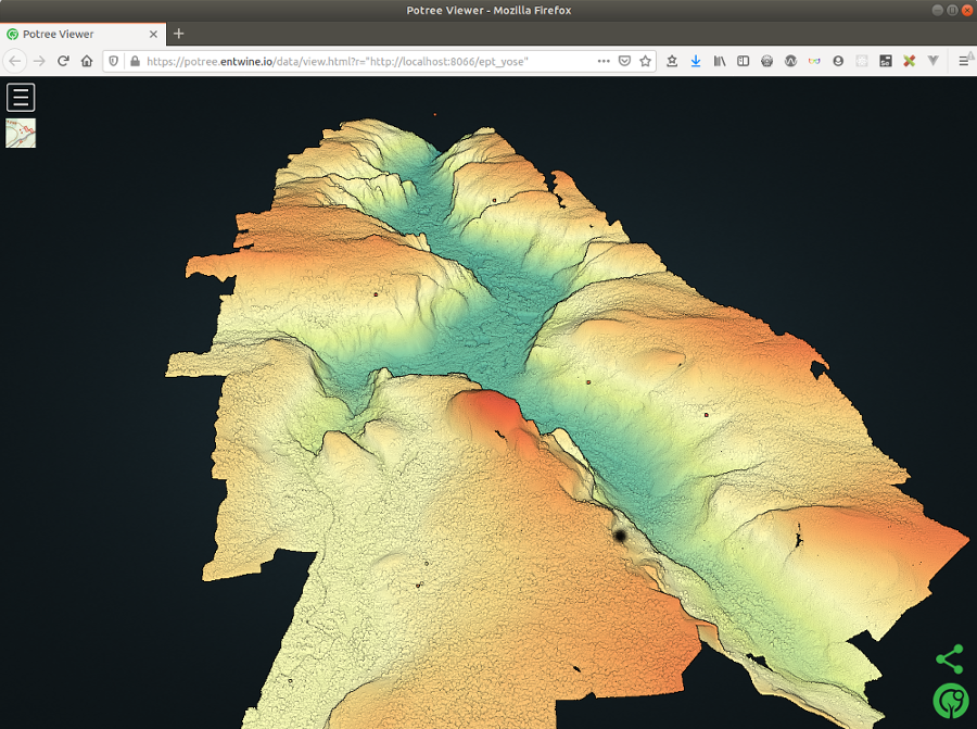
right view 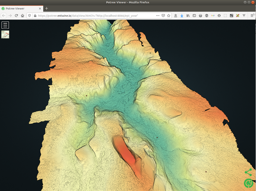
the dome 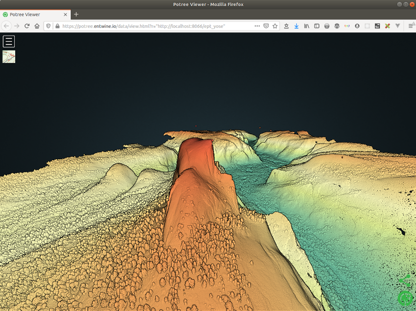
the dome 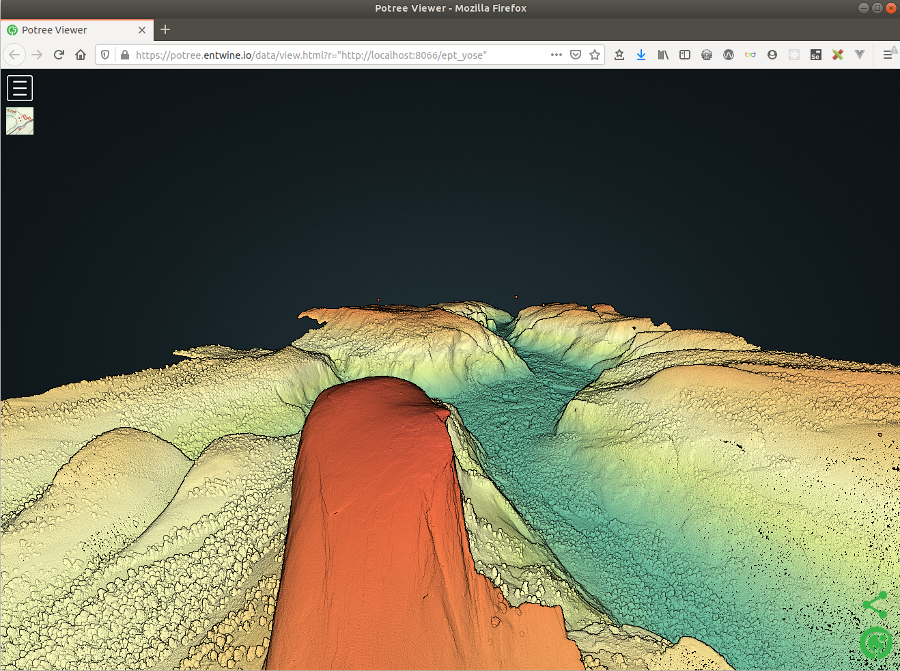
the dome 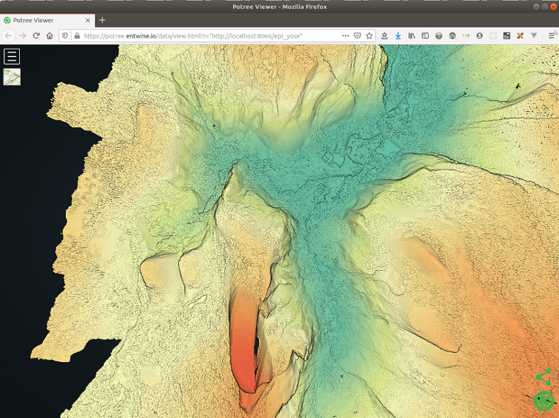
the dome 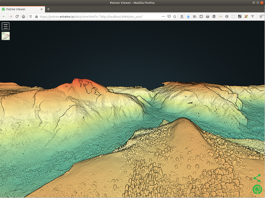
the dome 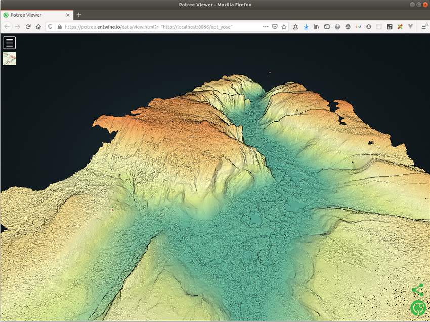
Glacier Point apron 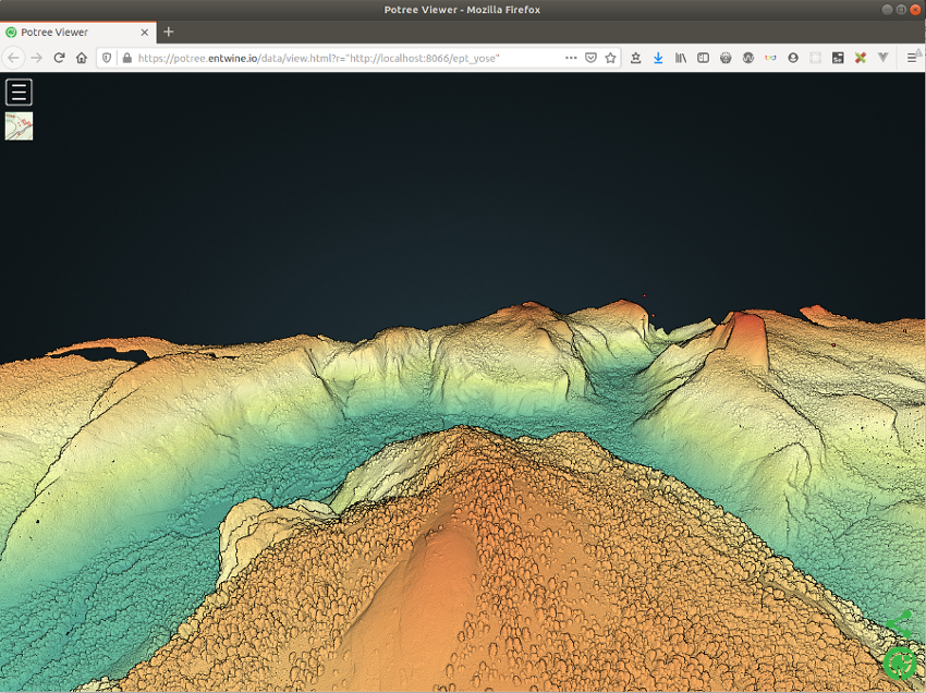
camp 4 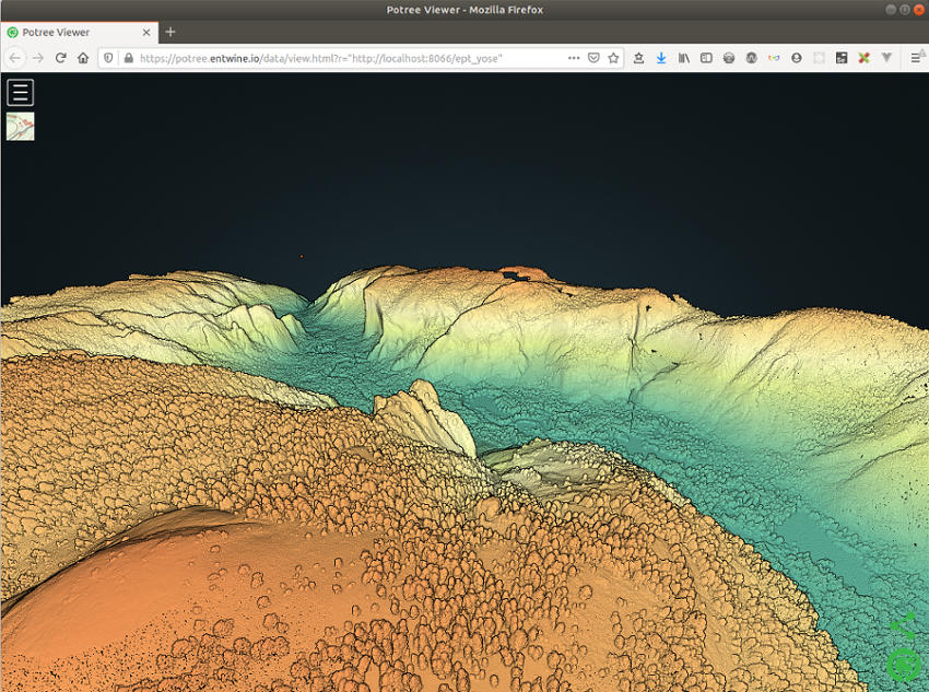
the sentinel 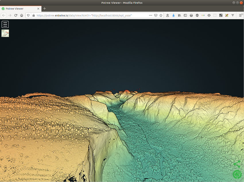
el capitan top 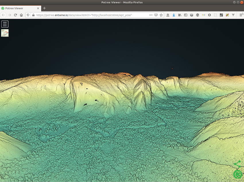
el capitan & three bro. 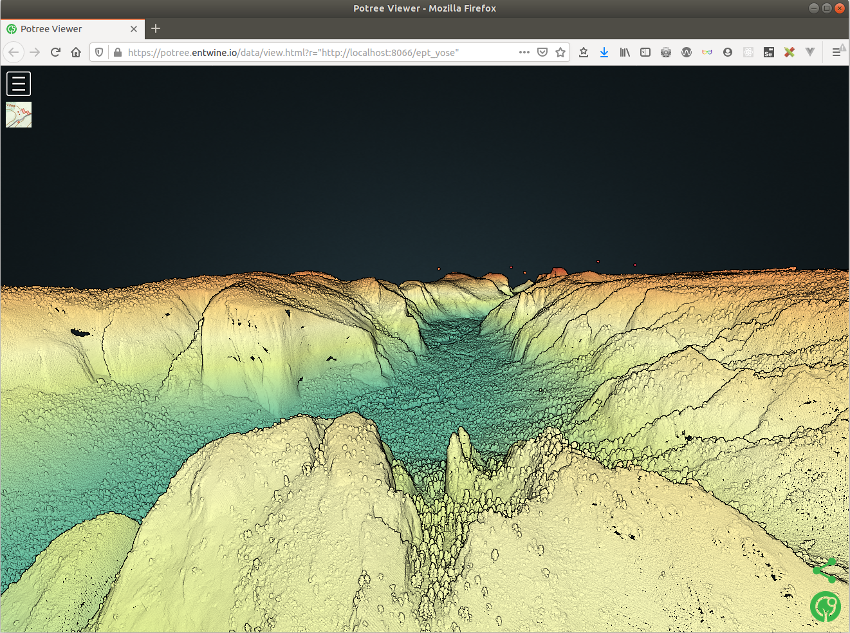
el capitan & cathedral sp 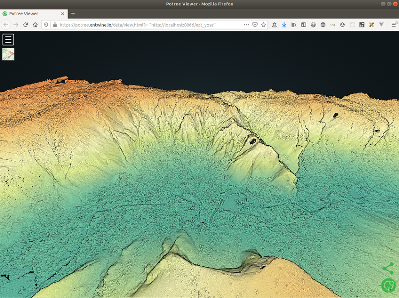
cathedral rocks & sp. 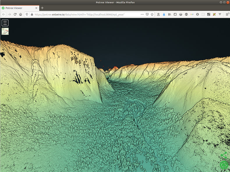
el capitan 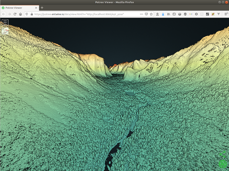
el capitan & bridalveil
The commonly used versions of the LAS format (1.2 and 1.3) have 8 classification categories pre-defined and can handle up to 32. For 1.4 see this document.
Visualize the points by point classification:
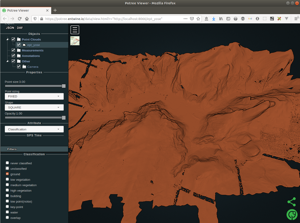
ground 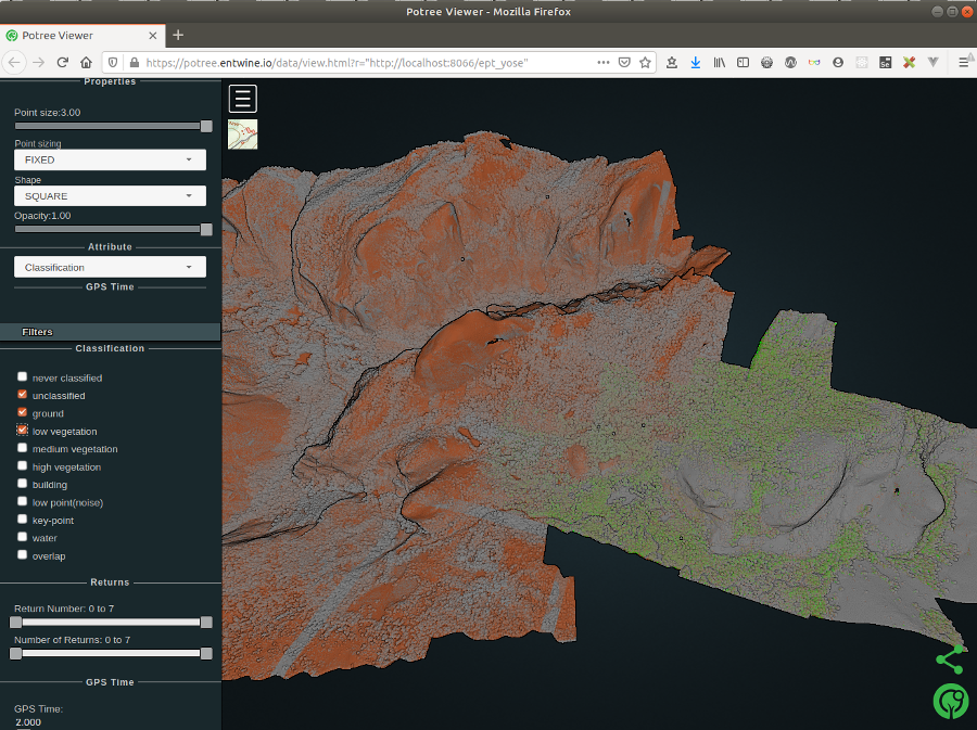
low vegetation 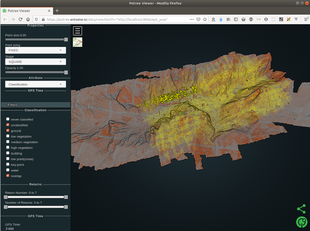
overlap 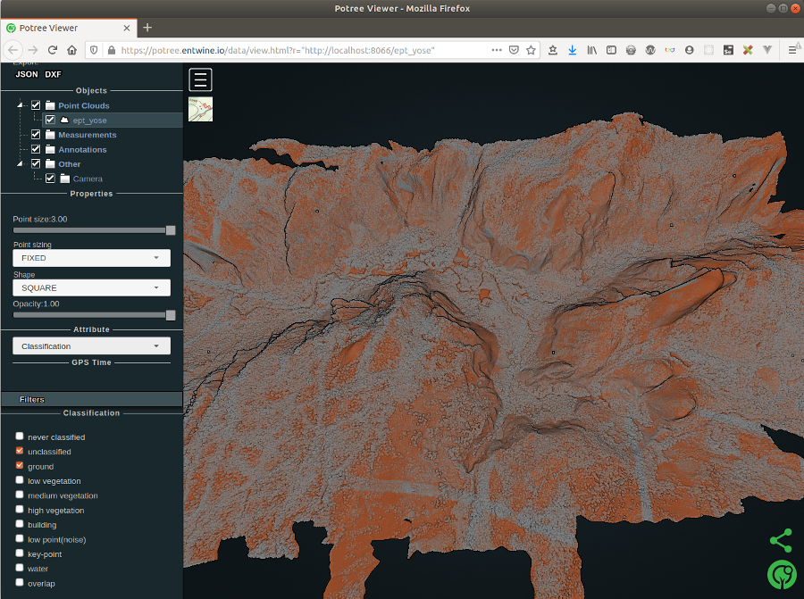
ground & unclassified
LiDAR data can contain significantly more information than x, y, and z values and may include, among others, the intensity of the returns, the point classification (if done), the number of returns, the time, and the source (flight line) of each point.
Intensity can be used as a substitute for aerial imagery when none is available.
Visualize the points by other attributes (intensity data, return number):
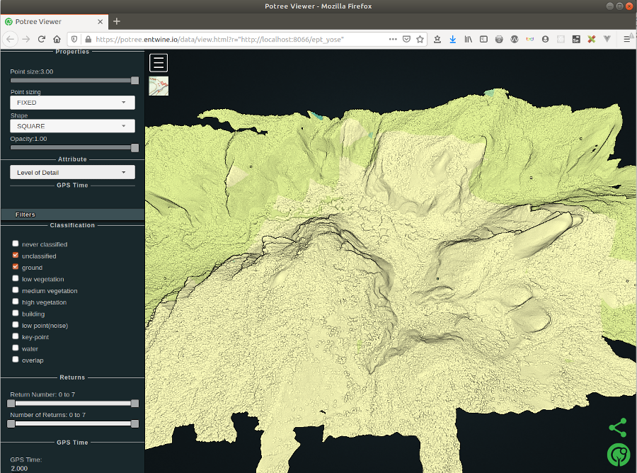
level of detail 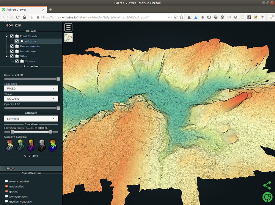
elevation 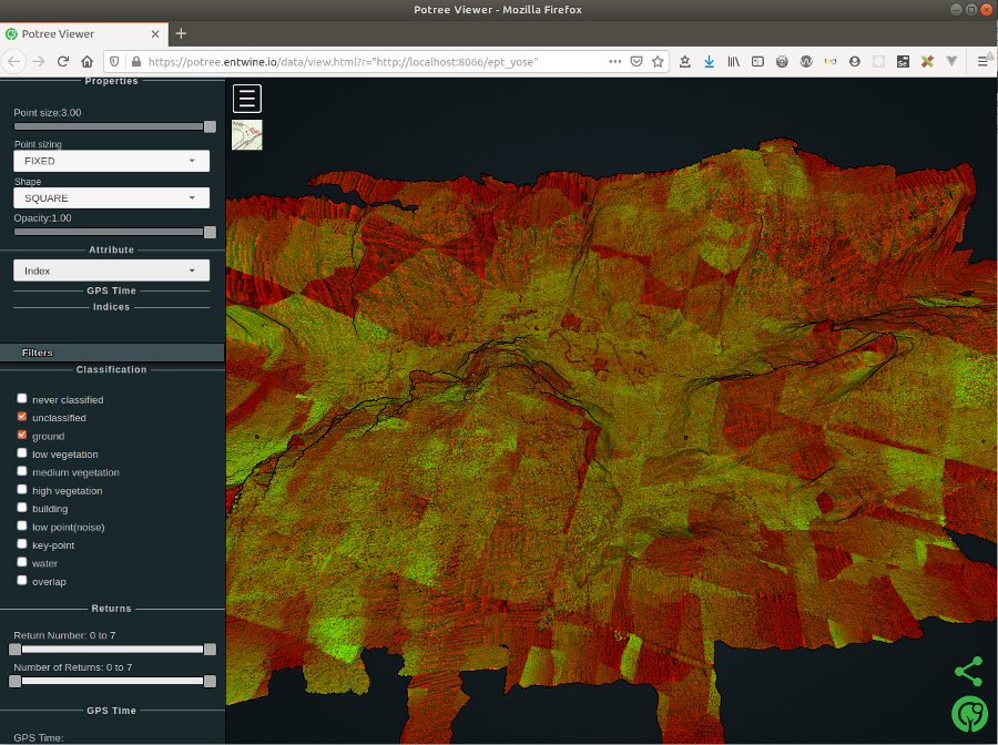
index 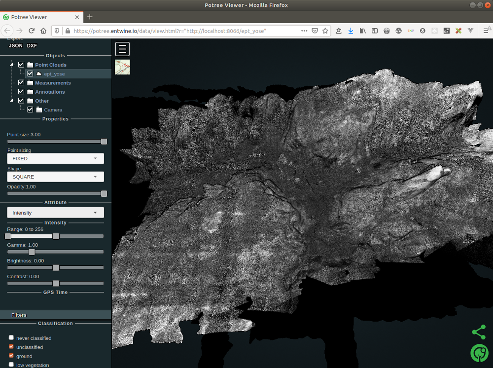
intensity 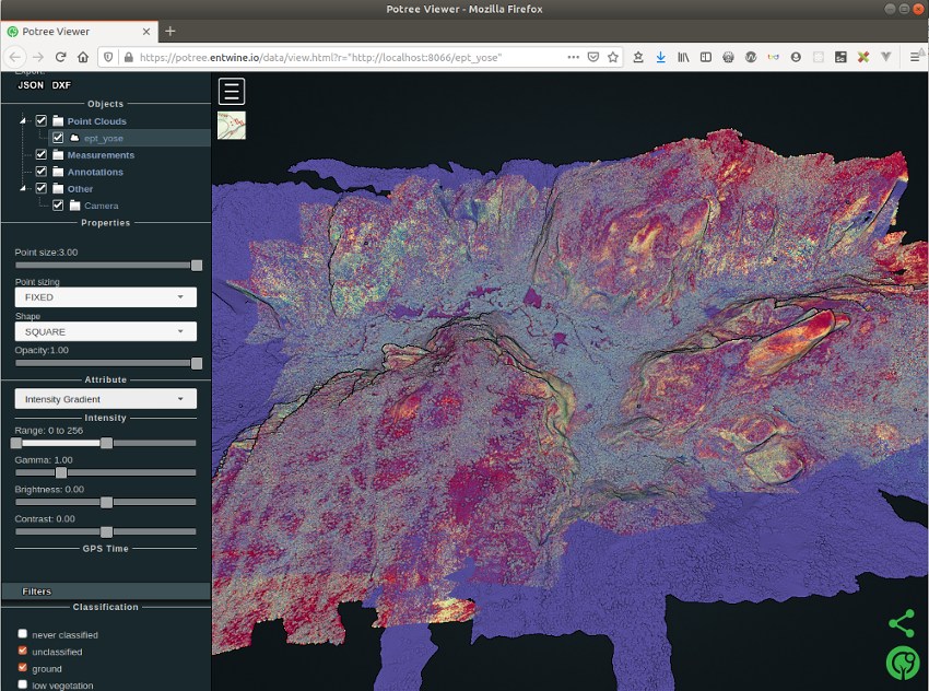
intensity gradient 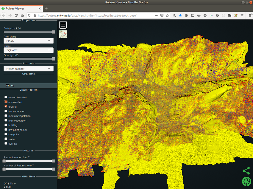
return number 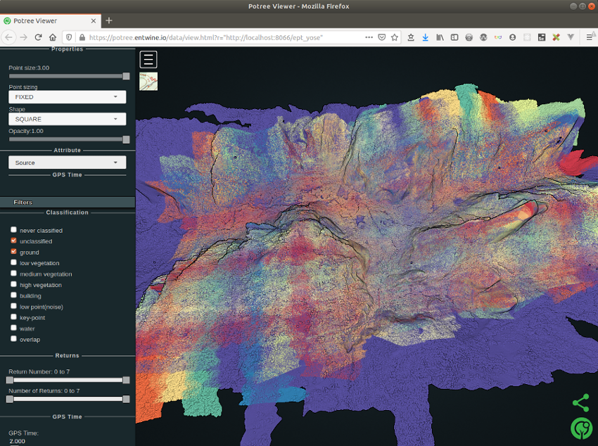
source
Visualize the points in Plasio, too.
# Visualise our local point cloud data in Plasio

xdg-open "http://dev.speck.ly/?s=0&r=ept://localhost:8066/ept_yose&c0s=local://color"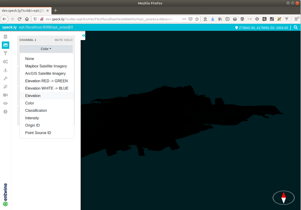
first view 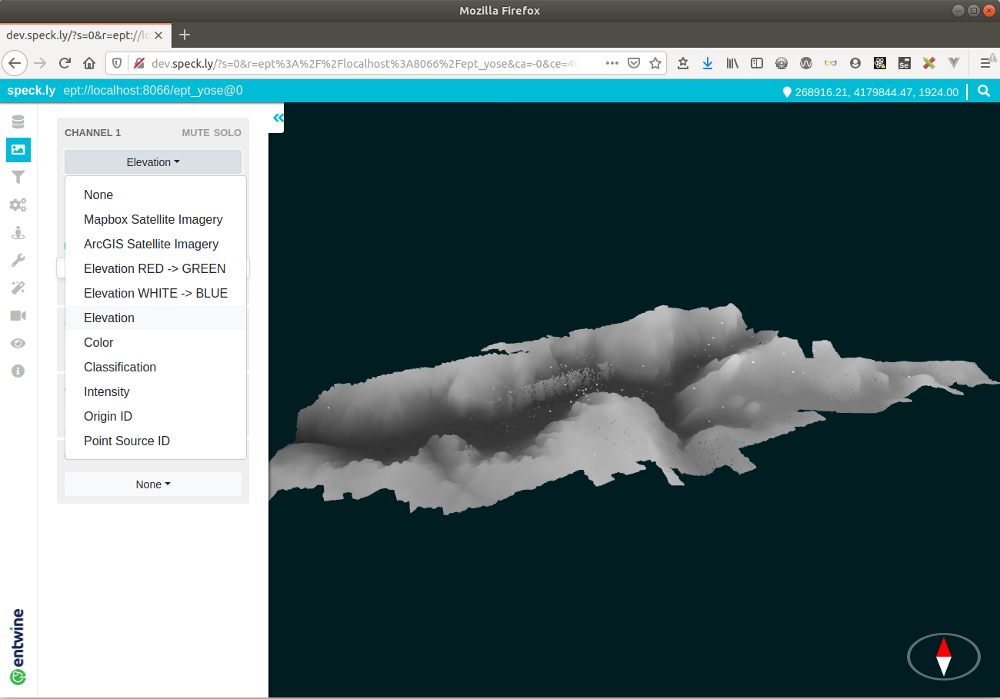
classify by elevation 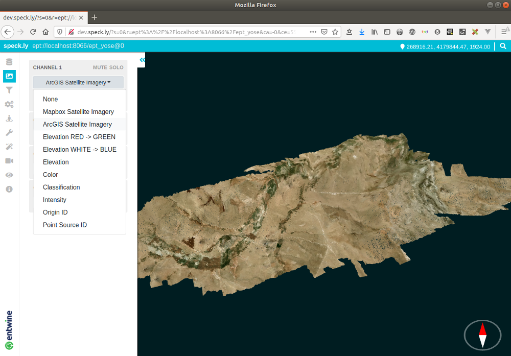
arcgis imagery overlap 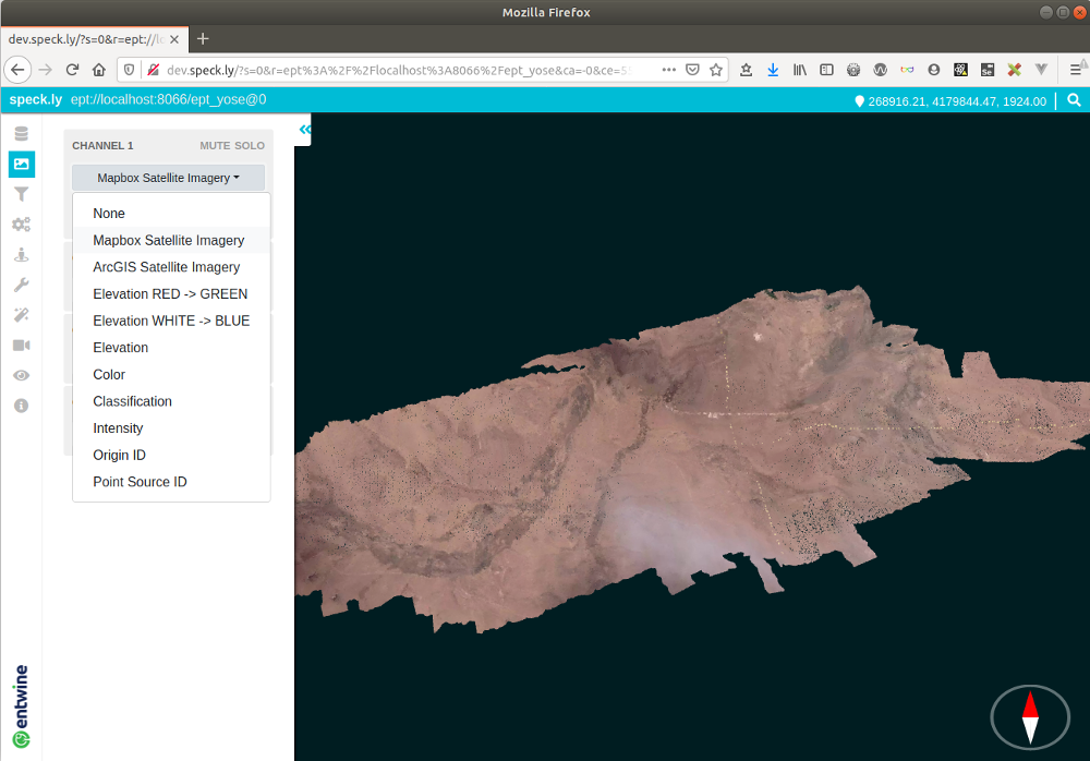
mapbox overlap 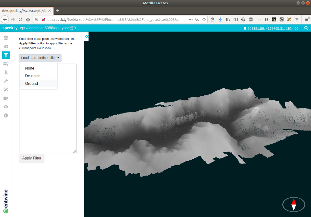
filter 
filter ground 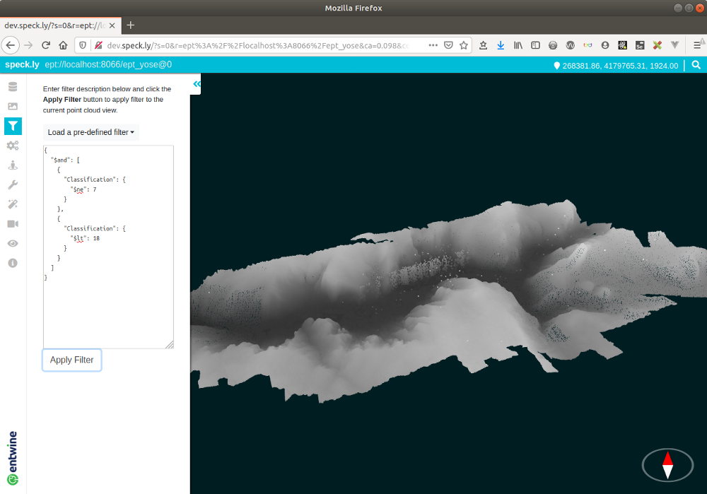
filter denoise 
z exaggeration 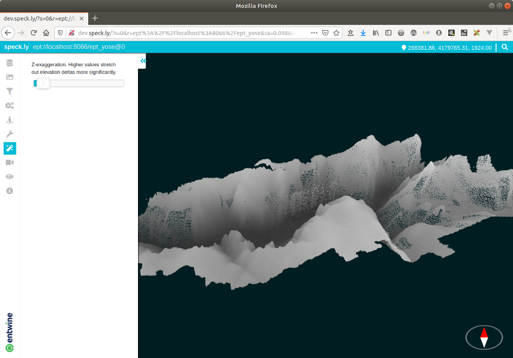
z exaggeration 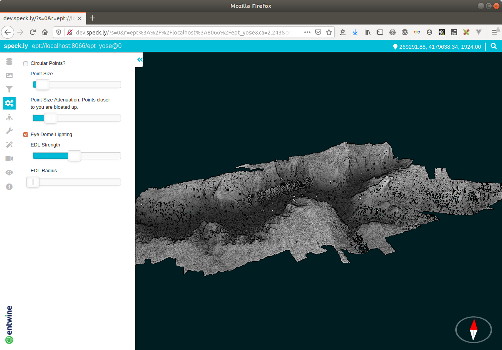
eye dome lighting 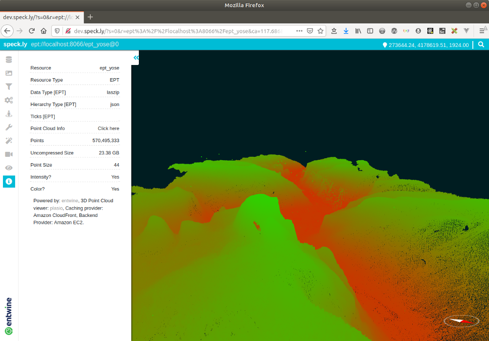
about
Finding the boundary (src)
Create a JSON file named entwine.json, containing the above code, then convert from EPT to LAZ using the pdal pipeline command.
{
    "pipeline": [
        {
            "type": "readers.ept",
            "filename":"ept_yose",
            "resolution": 5
        },
        {
            "type": "writers.las",
            "compression": "true",
            "minor_version": "2",
            "dataformat_id": "0",
            "filename":"temp_data/ept_yose_to_laz.laz"
        }
    ]
}
pdal pipeline entwine.json -v 7
pdal info temp_data/ept_yose_to_laz.laz | jq .stats.bbox.native.bbox
pdal info temp_data/ept_yose_to_laz.laz -p 0(new_clouds) myuser@comp:~/yose$ pdal pipeline entwine.json -v 7
(PDAL Debug) Debugging...
(pdal pipeline readers.ept Debug) Endpoint: ept_yose/
Got EPT info
SRS: PROJCS["NAD83 / UTM zone 11N",
GEOGCS["NAD83",
DATUM["North_American_Datum_1983",
SPHEROID["GRS 1980",6378137,298.257222101,
AUTHORITY["EPSG","7019"]],
AUTHORITY["EPSG","6269"]],
PRIMEM["Greenwich",0,
AUTHORITY["EPSG","8901"]],
UNIT["degree",0.0174532925199433,
AUTHORITY["EPSG","9122"]],
AUTHORITY["EPSG","4269"]],
PROJECTION["Transverse_Mercator"],
PARAMETER["latitude_of_origin",0],
PARAMETER["central_meridian",-117],
PARAMETER["scale_factor",0.9996],
PARAMETER["false_easting",500000],
PARAMETER["false_northing",0],
UNIT["metre",1,
AUTHORITY["EPSG","9001"]],
AXIS["Easting",EAST],
AXIS["Northing",NORTH],
AUTHORITY["EPSG","26911"]]
Root resolution: 177.734
Query resolution: 1
Actual resolution: 0.694275
Depth end: 9
Query bounds: ([-1.797693134862316e+308, 1.797693134862316e+308], [-1.797693134862316e+308, 1.797693134862316e+308], [-1.797693134862316e+308, 1.797693134862316e+308])
Threads: 4
(pdal pipeline readers.ept Debug) Registering dim X: double
(pdal pipeline readers.ept Debug) Registering dim Y: double
(pdal pipeline readers.ept Debug) Registering dim Z: double
(pdal pipeline readers.ept Debug) Registering dim Intensity: uint16_t
(pdal pipeline readers.ept Debug) Registering dim ReturnNumber: uint8_t
(pdal pipeline readers.ept Debug) Registering dim NumberOfReturns: uint8_t
(pdal pipeline readers.ept Debug) Registering dim ScanDirectionFlag: uint8_t
(pdal pipeline readers.ept Debug) Registering dim EdgeOfFlightLine: uint8_t
(pdal pipeline readers.ept Debug) Registering dim Classification: uint8_t
(pdal pipeline readers.ept Debug) Registering dim ScanAngleRank: float
(pdal pipeline readers.ept Debug) Registering dim UserData: uint8_t
(pdal pipeline readers.ept Debug) Registering dim PointSourceId: uint16_t
(pdal pipeline readers.ept Debug) Registering dim GpsTime: double
(pdal pipeline readers.ept Debug) Registering dim Red: uint16_t
(pdal pipeline readers.ept Debug) Registering dim Green: uint16_t
(pdal pipeline readers.ept Debug) Registering dim Blue: uint16_t
(pdal pipeline readers.ept Debug) Registering dim OriginId: uint32_t
(pdal pipeline Debug) Executing pipeline in stream mode.
(pdal pipeline readers.ept Debug) Overlap nodes: 12930
(pdal pipeline readers.ept Debug) Overlap points: 569789305
(pdal pipeline readers.ept Warning) 569789305 will be downloaded
(pdal pipeline readers.ept Debug) Streaming Data 1/12930: 0-0-0-0
(pdal pipeline readers.ept Debug) Points : 8369
(pdal pipeline readers.ept Debug) Streaming Data 2/12930: 1-0-0-0
(pdal pipeline readers.ept Debug) Points : 7140
[...]
(pdal pipeline readers.ept Debug) Streaming Data 12929/12930: 8-203-135-133
(pdal pipeline readers.ept Debug) Points : 20004
(pdal pipeline readers.ept Debug) Streaming Data 12930/12930: 8-209-129-128
(pdal pipeline readers.ept Debug) Points : 17287
(pdal pipeline writers.las Debug) Wrote 569789305 points to the LAS file
(new_clouds) myuser@comp:~/yose$ pdal info temp_data/ept_yose_to_laz.laz | jq .stats.bbox.native.bbox
{
"maxx": 285218.04,
"maxy": 4184499.99,
"maxz": 3100.04,
"minx": 262472.46,
"miny": 4174883.16,
"minz": 747.14
}
(new_clouds) myuser@comp:~/yose$ pdal info temp_data/ept_yose_to_laz.laz -p 0
{
"filename": "temp_data/ept_yose_to_laz.laz",
"pdal_version": "2.0.1 (git-version: 6600e6)",
"points":
{
"point":
{
"Classification": 2,
"EdgeOfFlightLine": 0,
"Intensity": 0,
"NumberOfReturns": 1,
"PointId": 0,
"PointSourceId": 0,
"ReturnNumber": 1,
"ScanAngleRank": 0,
"ScanDirectionFlag": 0,
"UserData": 0,
"X": 266469.82,
"Y": 4180471.6,
"Z": 2252.73
}
}
}
(new_clouds) myuser@comp:~/yose$
Get the boundary of the fitting polygon for the data as WKT or JSON.
pdal info temp_data/ept_yose_to_laz.laz --boundary(new_clouds) myuser@comp:~/yose$ pdal info temp_data/ept_yose_to_laz.laz --boundary
{
"boundary":
{
"area": 741660728.7,
"avg_pt_per_sq_unit": 3.904920938,
"avg_pt_spacing": 1.140894523,
"boundary": "POLYGON ((283713.94 4162551.0,294060.41 4192418.7,256123.35 4186445.1,256123.35 4174498.1,283713.94 4162551.0))",
"boundary_json": { "type": "Polygon", "coordinates": [ [ [ 283713.941809380019549, 4162550.982932080049068 ], [ 294060.414895010006148, 4192418.678045279812068 ], [ 256123.346914369991282, 4186445.1390226399526 ], [ 256123.346914369991282, 4174498.060977359768003 ], [ 283713.941809380019549, 4162550.982932080049068 ] ] ] },
"density": 0.7682613936,
"edge_length": 0,
"estimated_edge": 11947.07805,
"hex_offsets": "MULTIPOINT (0 0, -3448.82 5973.54, 0 11947.1, 6897.65 11947.1, 10346.5 5973.54, 6897.65 0)",
"sample_size": 5000,
"threshold": 15
},
"filename": "temp_data/ept_yose_to_laz.laz",
"pdal_version": "2.0.1 (git-version: 6600e6)"
}
(new_clouds) myuser@comp:~/yose$Get a vector geometry file using pdal tindex, the “tile index” command. Then view the file in QGIS.
# simple tindex
pdal tindex create --tindex temp_data/boundary.sqlite \
    --filespec temp_data/ept_yose_to_laz.laz \
    --t_srs "EPSG:26911" \
    -f SQLite
# set edge size for output
pdal tindex create --tindex temp_data/boundary2.sqlite \
    --filespec temp_data/ept_yose_to_laz.laz \
    --filters.hexbin.edge_size=10 \
    --filters.hexbin.threshold=1 \
    --t_srs "EPSG:26911" \
    -f SQLite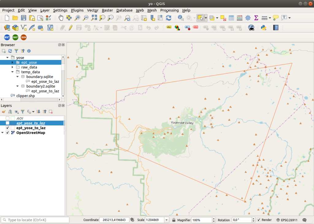
tindex boundary in QGIS 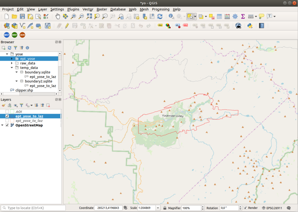
fine boundary


Or use Hexbin to output the boundary of actual points in point buffer, not just rectangular extents. Create a file named hexbin-pipeline.json and populate it with the code below, then run pdal pipeline.
[
    "temp_data/ept_yose_to_laz.laz",
    {
        "type" : "filters.hexbin"
    }
]
pdal pipeline hexbin-pipeline.json --metadata hexbin-out.json
pdal info --boundary temp_data/ept_yose_to_laz.laz(new_clouds) myuser@comp:~/yose$ tree -L 1
.
├── entwine.json
├── ept_yose
├── hexbin-out.json
├── hexbin-pipeline.json
├── raw_data
└── temp_data
3 directories, 3 files
(new_clouds) myuser@comp:~/yose$ pdal pipeline hexbin-pipeline.json --metadata hexbin-out.json
(new_clouds) myuser@comp:~/yose$ pdal info --boundary temp_data/ept_yose_to_laz.laz
{
"boundary":
{
"area": 741660728.7,
"avg_pt_per_sq_unit": 3.904920938,
"avg_pt_spacing": 1.140894523,
"boundary": "POLYGON ((283713.94 4162551.0,294060.41 4192418.7,256123.35 4186445.1,256123.35 4174498.1,283713.94 4162551.0))",
"boundary_json": { "type": "Polygon", "coordinates": [ [ [ 283713.941809380019549, 4162550.982932080049068 ], [ 294060.414895010006148, 4192418.678045279812068 ], [ 256123.346914369991282, 4186445.1390226399526 ], [ 256123.346914369991282, 4174498.060977359768003 ], [ 283713.941809380019549, 4162550.982932080049068 ] ] ] },
"density": 0.7682613936,
"edge_length": 0,
"estimated_edge": 11947.07805,
"hex_offsets": "MULTIPOINT (0 0, -3448.82 5973.54, 0 11947.1, 6897.65 11947.1, 10346.5 5973.54, 6897.65 0)",
"sample_size": 5000,
"threshold": 15
},
"filename": "temp_data/ept_yose_to_laz.laz",
"pdal_version": "2.0.1 (git-version: 6600e6)"
}
(new_clouds) myuser@comp:~/yose$Cropping
pdal translate -i temp_data/ept_yose_to_laz.laz \
   -o temp_data/ept_yose_cropped.laz \
   --readers.las.spatialreference="EPSG:26911" -f crop  \
   --filters.crop.polygon="MultiPolygon (((279868.59169999975711107 4180921.18200000002980232, 279928.44170000031590462 4180963.2715000007301569, 280010.16590000037103891 4181071.09950000047683716, 280088.36830000020563602 4181131.01630000025033951, 280179.64120000042021275 4181168.09600000083446503, 280277.47350000031292439 4181179.69329999946057796, 280374.88599999994039536 4181164.98100000061094761, 280505.14730000030249357 4181096.37509999983012676, 280624.1380000002682209 4180940.14929999969899654, 280740.60049999970942736 4180849.40240000002086163, 281026.84020000044256449 4180775.61299999989569187, 281322.41069999989122152 4180774.36350000090897083, 281752.026999999769032 4180868.35329999960958958, 282136.17349999956786633 4180892.94510000012814999, 282376.50169999990612268 4180879.24520000070333481, 283137.27850000001490116 4180789.59530000016093254, 283519.64089999999850988 4180775.78930000029504299, 283901.73670000024139881 4180782.89690000005066395, 284282.35400000028312206 4180749.79539999924600124, 284612.66909999959170818 4180677.4398999996483326, 284700.1507999999448657 4180629.45500000007450581, 284776.20710000023245811 4180564.87130000069737434, 284862.24210000038146973 4180442.79470000043511391, 284897.48809999972581863 4180349.44950000010430813, 284913.25989999994635582 4180250.9261000007390976, 284908.91430000029504299 4180151.24300000071525574, 284842.28699999954551458 4180078.55729999952018261, 284722.16629999969154596 4179992.63010000064969063, 284536.23900000005960464 4179928.97199999913573265, 284207.49220000021159649 4179913.31729999929666519, 283795.92509999964386225 4179930.56849999912083149, 283665.24849999975413084 4179903.53820000030100346, 283514.55730000045150518 4179809.92980000004172325, 283418.81630000006407499 4179649.01349999941885471, 283283.02780000027269125 4179520.08770000003278255, 283160.93369999993592501 4179450.31059999950230122, 282936.66210000030696392 4179368.4517000000923872, 282794.24270000029355288 4179341.74799999967217445, 282649.36809999961405993 4179338.97049999982118607, 282458.56089999992400408 4179394.70519999973475933, 282260.64809999987483025 4179413.25980000011622906, 282111.86539999954402447 4179402.32010000012814999, 281966.16150000039488077 4179370.28329999931156635, 281559.90639999974519014 4179201.70729999989271164, 281147.33420000039041042 4178950.64990000054240227, 280968.37999999988824129 4178881.02889999933540821, 280736.09100000001490116 4178820.82489999942481518, 280400.0669999998062849 4178792.96199999935925007, 280014.29299999959766865 4178797.3063999991863966, 278908.24579999968409538 4178924.33180000074207783, 278290.53880000021308661 4178971.92119999974966049, 278156.83820000011473894 4178954.69590000063180923, 278032.64759999979287386 4178902.26290000043809414, 277988.09619999956339598 4178764.92549999989569187, 277994.86450000014156103 4178620.70150000043213367, 278008.56709999963641167 4178574.32320000045001507, 278074.37609999999403954 4178501.97900000028312206, 278156.43620000034570694 4178448.77510000020265579, 278293.27350000012665987 4178395.75479999929666519, 278323.85460000019520521 4178357.02850000001490116, 278335.52049999963492155 4178309.0823999997228384, 278326.14969999995082617 4178260.63539999909698963, 278297.44629999995231628 4178220.49770000018179417, 278254.63009999971836805 4178195.96820000000298023, 277924.5530000003054738 4178129.56739999912679195, 277699.45299999974668026 4178044.40650000050663948, 277528.98880000039935112 4177954.78040000051259995, 277082.19359999988228083 4177666.37590000033378601, 276645.08420000039041042 4177455.26209999993443489, 276279.17659999988973141 4177324.94659999944269657, 275807.47439999971538782 4177213.72460000030696392, 275718.1732999999076128 4177177.3385000005364418, 275603.77880000043660402 4177089.38739999942481518, 275545.66610000003129244 4177012.43569999933242798, 275505.29370000027120113 4176924.86449999921023846, 275474.71459999959915876 4176788.77979999966919422, 275427.71499999985098839 4176710.5234999991953373, 275315.19739999994635582 4176634.00070000067353249, 274789.14869999978691339 4176527.06990000046789646, 274225.01790000032633543 4176341.23540000058710575, 274128.89580000005662441 4176324.24960000067949295, 273982.70590000040829182 4176327.54040000028908253, 273646.84949999954551458 4176403.94539999961853027, 273351.11270000040531158 4176436.10769999958574772, 273053.63250000029802322 4176436.54979999922215939, 272671.47539999987930059 4176395.39719999954104424, 272540.48500000033527613 4176357.11119999922811985, 272417.11699999962002039 4176298.76190000027418137, 272273.1931999996304512 4176168.79160000011324883, 272145.3738000001758337 4176091.37989999912679195, 271819.73209999967366457 4176001.75960000045597553, 271651.38109999988228083 4175918.6375999990850687, 271560.803999999538064 4175894.2040999997407198, 271466.98979999963194132 4175893.86669999919831753, 271376.23929999954998493 4175917.64809999987483025, 271219.38040000014007092 4176016.1919999998062849, 271091.88989999983459711 4176060.94079999998211861, 270957.40720000024884939 4176074.0056999996304512, 270769.66870000027120113 4176044.83459999971091747, 270403.15629999991506338 4175945.53749999962747097, 270055.17619999963790178 4175793.54680000059306622, 268938.80389999970793724 4175411.07379999943077564, 268043.12220000009983778 4175170.76899999938905239, 267708.31740000005811453 4175140.02459999918937683, 267401.40010000020265579 4175190.29560000076889992, 267202.97979999985545874 4175177.59019999951124191, 266956.83810000028461218 4175210.66349999979138374, 266679.76580000016838312 4175319.71700000017881393, 266319.58289999980479479 4175569.37979999929666519, 266187.01329999975860119 4175625.47140000015497208, 266049.48419999983161688 4175654.33049999922513962, 265870.71820000000298023 4175637.71160000003874302, 265649.31809999980032444 4175552.66440000012516975, 265504.33040000032633543 4175525.58860000036656857, 265356.9386999998241663 4175531.08390000090003014, 265175.46769999992102385 4175578.3489999994635582, 265041.26970000006258488 4175575.28830000013113022, 264955.16119999997317791 4175549.98079999908804893, 264846.52969999983906746 4175475.69999999925494194, 264764.72570000030100346 4175459.55550000071525574, 264649.72790000028908253 4175505.15029999986290932, 264506.85259999986737967 4175698.29659999907016754, 264396.17100000008940697 4175751.5113999992609024, 264313.70639999955892563 4175748.56750000081956387, 264231.3477999996393919 4175698.35909999907016754, 264092.8892000000923872 4175657.51620000042021275, 263625.97840000037103891 4175691.59559999965131283, 263442.43840000033378601 4175663.5859999991953373, 263171.81300000008195639 4175575.2642000000923872, 263027.82880000025033951 4175568.65049999952316284, 262860.85589999984949827 4175629.9789000004529953, 262710.32820000033825636 4175724.75500000081956387, 262624.11699999962002039 4175954.87390000000596046, 262580.73089999984949827 4176146.68600000068545341, 262560.79399999976158142 4176342.33039999939501286, 262533.05700000002980232 4177603.30040000006556511, 262530.41119999997317791 4178664.28170000016689301, 262541.18049999978393316 4178760.50180000066757202, 262577.43200000002980232 4178850.27989999949932098, 262673.27680000010877848 4178958.64629999920725822, 263035.80339999962598085 4179196.30690000019967556, 263575.4786999998614192 4179593.83640000037848949, 263744.11419999971985817 4179675.80330000072717667, 263879.55410000029951334 4179714.02930000051856041, 264462.93730000033974648 4179770.44050000049173832, 264896.71669999975711107 4179861.34429999999701977, 266329.83540000021457672 4180362.91009999997913837, 267437.02199999988079071 4180643.22800000011920929, 268560.03679999988526106 4181013.64890000037848949, 268891.11189999990165234 4181092.05629999935626984, 269323.79739999957382679 4181167.54499999992549419, 269797.51669999957084656 4181312.06140000000596046, 269981.09269999992102385 4181386.84960000030696392, 270015.27680000010877848 4181419.51830000057816505, 270080.25030000042170286 4181544.18979999981820583, 270101.82290000002831221 4181727.36219999939203262, 270151.0790999997407198 4181853.48240000009536743, 270260.85099999979138374 4182000.3688999991863966, 270413.84570000041276217 4182115.3818999994546175, 270816.92100000008940697 4182243.27209999971091747, 271170.85649999976158142 4182448.30770000070333481, 271395.59949999954551458 4182495.37590000033378601, 271528.28940000012516975 4182543.71580000035464764, 271901.82440000027418137 4182767.3624000009149313, 272266.33440000005066395 4182920.85500000044703484, 272871.12090000044554472 4183090.02199999988079071, 273445.47140000015497208 4183301.64589999988675117, 273626.80310000013560057 4183331.28940000012516975, 273957.74370000045746565 4183340.05670000053942204, 274192.61380000039935112 4183395.4232999999076128, 274325.55979999992996454 4183453.24960000067949295, 274509.52219999954104424 4183609.28030000068247318, 274752.51449999958276749 4183748.71160000003874302, 274876.54509999975562096 4183788.90670000016689301, 275005.93350000027567148 4183795.86840000003576279, 275087.33459999971091747 4183820.33669999986886978, 275206.59470000024884939 4183953.28179999999701977, 275287.50019999966025352 4184002.48369999974966049, 275425.20820000022649765 4184027.77659999951720238, 275662.13999999966472387 4184023.51080000028014183, 275757.83399999979883432 4184046.1602999996393919, 275886.60450000036507845 4184117.3551000002771616, 276019.99110000021755695 4184244.83650000020861626, 276186.48469999991357327 4184324.35610000044107437, 276323.16789999976754189 4184347.54299999959766865, 276975.34449999965727329 4184347.60639999993145466, 277101.3101000003516674 4184284.97100000083446503, 277203.97580000013113022 4184142.3596000000834465, 277329.89809999987483025 4184091.9488999992609024, 277429.1294999998062849 4184097.31279999949038029, 277571.31300000008195639 4184132.61040000058710575, 277834.92939999978989363 4184074.49129999987781048, 277921.25439999997615814 4184090.89670000039041042, 277955.71059999987483025 4184123.3255000002682209, 278042.84530000016093254 4184158.3278999999165535, 278136.12160000018775463 4184147.50430000014603138, 278327.45309999957680702 4184018.60669999942183495, 278441.71389999985694885 4183874.75879999995231628, 278513.67740000039339066 4183715.93520000018179417, 278537.34190000034868717 4183496.52710000053048134, 278590.2911999998614192 4183421.01679999940097332, 278629.07400000002235174 4183395.40550000034272671, 278719.31070000026375055 4183376.35899999924004078, 278894.74370000045746565 4183443.30260000005364418, 278990.59460000041872263 4183448.85459999926388264, 279121.61349999997764826 4183391.65839999914169312, 279182.70720000006258488 4183317.59229999966919422, 279231.0014000004157424 4183184.35359999909996986, 279256.08019999973475933 4183046.24660000018775463, 279253.78749999962747097 4182859.27080000005662441, 279232.19369999971240759 4182771.06079999916255474, 279180.93350000027567148 4182699.09429999999701977, 278982.67229999974370003 4182589.11009999923408031, 278904.51470000017434359 4182470.57840000092983246, 278891.41299999970942736 4182376.20099999941885471, 278950.48570000007748604 4182003.33000000007450581, 279005.65409999992698431 4181933.59369999915361404, 279172.79229999985545874 4181881.6640000008046627, 279261.53560000006109476 4181786.94549999944865704, 279334.78380000032484531 4181477.50669999979436398, 279372.97140000015497208 4181110.88519999943673611, 279421.44489999953657389 4180979.39049999974668026, 279491.86830000020563602 4180937.43679999932646751, 279570.94730000011622906 4180915.84830000065267086, 279740.76750000007450581 4180901.07990000024437904, 279868.59169999975711107 4180921.18200000002980232)))"
pdal info temp_data/ept_yose_cropped.laz --boundary
(new_clouds) myuser@comp:~/yose$ pdal info temp_data/ept_yose_cropped.laz --boundary
{
"boundary":
{
"area": 716413798.1,
"avg_pt_per_sq_unit": 3.852125713,
"avg_pt_spacing": 1.133155728,
"boundary": "POLYGON ((283415.37 4162704.7,293584.21 4192059.6,256298.44 4186188.6,256298.44 4174446.6,283415.37 4162704.7))",
"boundary_json": { "type": "Polygon", "coordinates": [ [ [ 283415.366322420013603, 4162704.652427020017058 ], [ 293584.212115879985504, 4192059.58171531977132 ], [ 256298.444206549989758, 4186188.595857659820467 ], [ 256298.444206549989758, 4174446.624142339918762 ], [ 283415.366322420013603, 4162704.652427020017058 ] ] ] },
"density": 0.7787907833,
"edge_length": 0,
"estimated_edge": 11741.97172,
"hex_offsets": "MULTIPOINT (0 0, -3389.62 5870.99, 0 11742, 6779.23 11742, 10168.8 5870.99, 6779.23 0)",
"sample_size": 5000,
"threshold": 15
},
"filename": "temp_data/ept_yose_cropped.laz",
"pdal_version": "2.0.1 (git-version: 6600e6)"
}
(new_clouds) myuser@comp:~/yose$Clipping data with polygons (src)
TODO
{
    "pipeline": [
        "temp_data/ept_yose_to_laz.laz",
        {
            "column": "CLS",
            "datasource": "clipper.geojson",
            "dimension": "Classification",
            "type": "filters.overlay"
        },
        {
            "limits": "Classification[6:6]",
            "type": "filters.range"
        },
        "temp_data/ept_yose_clipped.laz"
    ]
}
pdal pipeline clipping.json --nostreamColorizing points with imagery (src)
I have used free aerial data downloaded from NAIP (National Agriculture Imagery Program), merged in a vrt file.
{
    "pipeline": [
        "temp_data/ept_yose_to_laz.laz",
        {
            "type": "filters.colorization",
            "raster": "aerial.vrt"
        },
        {
            "type": "filters.range",
            "limits": "Red[1:]"
        },
        {
            "type": "writers.las",
            "compression": "true",
            "minor_version": "2",
            "dataformat_id": "3",
            "filename":"temp_data/yose-colored.laz"
        }
    ]
}
pdal pipeline colorize.json
ls -lah temp_data/yose-colored.laz(new_clouds) myuser@comp:~/yose$ pdal pipeline colorize.json
(new_clouds) myuser@comp:~/yose$ ls -lah temp_data/yose-colored.laz
-rw-r--r-- 1 myuser myuser 3,5G feb 21 21:01 yose-colored.laz
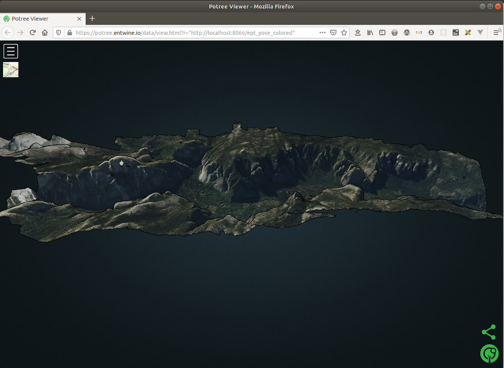
(new_clouds) myuser@comp:~/yose$Now let’s try to visualize the LAZ file in Potree creating an Entwine EPT file.
entwine build -i temp_data/yose-colored.laz -o ept_yose_colored --srs "EPSG:26911"
tree ept_yose_colored/ | head -10
tree ept_yose_colored/ | tail -10
(new_clouds) myuser@comp:~/yose$ entwine build -i temp_data/yose-colored.laz -o ept_yose_colored --srs "EPSG:26911"
Scanning input
1/1: temp_data/yose-colored.laz
Entwine Version: 2.1.0
EPT Version: 1.0.0
Input:
File: temp_data/yose-colored.laz
Total points: 569,789,305
Density estimate (per square unit): 2.60487
Threads: [1, 7]
Output:
Path: ept_yose_colored/
Data type: laszip
Hierarchy type: json
Sleep count: 2,097,152
Scale: 0.01
Offset: (273845, 4179692, 1924)
Metadata:
SRS: EPSG:26911
Bounds: [(262472, 4174883, 747), (285219, 4184500, 3101)]
Cube: [(262471, 4168317, -9451), (285221, 4191067, 13299)]
Storing dimensions: [
X:int32, Y:int32, Z:int32, Intensity:uint16, ReturnNumber:uint8,
NumberOfReturns:uint8, ScanDirectionFlag:uint8,
EdgeOfFlightLine:uint8, Classification:uint8, ScanAngleRank:float,
UserData:uint8, PointSourceId:uint16, GpsTime:double, Red:uint16,
Green:uint16, Blue:uint16, OriginId:uint32
]
Build parameters:
Span: 128
Resolution 2D: 128 * 128 = 16,384
Resolution 3D: 128 * 128 * 128 = 2,097,152
Maximum node size: 65,536
Minimum node size: 16,384
Cache size: 64
Adding 0 - temp_data/yose-colored.laz
Pushes complete - joining...
00:10 - 1% - 7,020,544 - 2,527(2,527)M/h - 17W - 0R - 146A
00:20 - 2% - 13,324,288 - 2,398(2,269)M/h - 119W - 3R - 148A
00:30 - 3% - 17,936,384 - 2,152(1,660)M/h - 91W - 14R - 161A
[...]
24:30 - 97% - 551,444,480 - 1,350(1,335)M/h - 152W - 38R - 230A
24:40 - 97% - 554,762,240 - 1,349(1,194)M/h - 167W - 46R - 202A
24:50 - 98% - 558,350,336 - 1,349(1,291)M/h - 89W - 37R - 249A
25:00 - 98% - 561,094,656 - 1,346(987)M/h - 184W - 51R - 203A
25:10 - 99% - 564,207,616 - 1,345(1,120)M/h - 97W - 46R - 258A
25:20 - 100% - 567,181,312 - 1,343(1,070)M/h - 101W - 52R - 319A
25:30 - 100% - 569,446,400 - 1,339(815)M/h - 245W - 63R - 238A
Done 0
Reawakened: 6238
Saving registry...
Saving metadata...
Index completed in 25:33.
Save complete.
Points inserted: 569,789,305
(new_clouds) myuser@comp:~/yose$ tree ept_yose_colored/ | head -10
ept_yose_colored/
├── ept-build.json
├── ept-data
│ ├── 0-0-0-0.laz
│ ├── 1-0-0-0.laz
│ ├── 1-0-0-1.laz
│ ├── 1-0-1-0.laz
│ ├── 1-0-1-1.laz
│ ├── 1-1-0-0.laz
│ ├── 1-1-0-1.laz
(new_clouds) myuser@comp:~/yose$
(new_clouds) myuser@comp:~/yose$ tree ept_yose_colored/ | tail -10
│ ├── 8-99-98-132.laz
│ └── 8-99-99-132.laz
├── ept-hierarchy
│ └── 0-0-0-0.json
├── ept.json
└── ept-sources
├── 0.json
└── list.json
3 directories, 13385 files
(new_clouds) myuser@comp:~/yose$Now, we can view the file in Potree:
http-server -p 8066 --cors
xdg-open "http://potree.entwine.io/data/view.html?r=http://localhost:8066/ept_yose_colored"


Removing noise (src)
Use PDAL to remove unwanted noise. Create a file named denoise.json and populate it with the following code, then run pdal pipeline.
{
    "pipeline": [
        "raw_data/points_little_yose.laz",
        {
            "type": "filters.outlier",
            "method": "statistical",
            "multiplier": 3,
            "mean_k": 8
        },
        {
            "type": "filters.range",
            "limits": "Classification![7:7],Z[-100:3000]"
        },
        {
            "type": "writers.las",
            "compression": "true",
            "minor_version": "2",
            "dataformat_id": "0",
            "filename":"temp_data/clean.laz"
        }
    ]
}
pdal pipeline denoise.json(new_clouds) myuser@comp:~/yose$ pdal pipeline denoise.json
(new_clouds) myuser@comp:~/yose$ tree temp_data/
temp_data/
├── boundary2.sqlite
├── boundary.sqlite
├── clean.laz
├── ept_yose_cropped.laz
├── ept_yose_to_laz.laz
└── points_little_yose_wgs84.laz
0 directories, 6 files
(new_clouds) myuser@comp:~/yose$Visualizing acquisition density (src)
Generate a density surface to summarize acquisition quality, and visualize it in QGIS, applying a gradient color ramp and using the count attribute.
pdal density raw_data/points_little_yose.laz  \
    -o temp_data/density.sqlite \
    -f SQLite
acquisition density
Thinning (src)
Subsample or thin point cloud data, to accelerate processing (less data), normalize point density, or ease visualization.
pdal translate raw_data/points_little_yose.laz \
    temp_data/thin.laz \
    sample --filters.sample.radius=20
tree temp_data/
(new_clouds) myuser@comp:~/yose$ pdal translate raw_data/points_little_yose.laz \
> temp_data/thin.laz \
> sample --filters.sample.radius=20
(new_clouds) myuser@comp:~/yose$ tree temp_data/
temp_data/
├── boundary2.sqlite
├── boundary.sqlite
├── clean.laz
├── density.sqlite
├── ept_yose_cropped.laz
├── ept_yose_to_laz.laz
├── points_little_yose_wgs84.laz
└── thin.laz
0 directories, 8 files
(new_clouds) myuser@comp:~/yose$Creating tiles (tile)
Before running the next commands, we will have to split the files into tiles. Then run the command in batches, because we can run out of memory if the file was too large, with the error PDAL: std::bad_allocfor example.
We will start from the beginning, and use the LAS files from the raw_data folder. First, we reproject points_little_yose.las from “EPSG:32611” to “EPSG:26911” (from “WGS 84 / UTM zone 11N” to “NAD83 / UTM zone 11N”).
WGS 84 / UTM zone 11N - EPSG:32611 - EPSG.io
epsg.io › 32611
Traducerea acestei pagini
EPSG:32611 Projected coordinate system for Between 120°W and 114°W, northern hemisphere between equator and 84°N, onshore and offshore.

NAD83 / UTM zone 11N - EPSG:26911 - EPSG.io
epsg.io › 26911
Traducerea acestei pagini
EPSG:26911 Projected coordinate system for North America - between 120°W and 114°W - onshore and offshore.
pdal translate raw_data/points_little_yose.las \
raw_data/points_little_yose_nad83.las reprojection \
--filters.reprojection.in_srs="EPSG:32611" \
--filters.reprojection.out_srs="EPSG:26911"Then we move the files we need for making tiles in a new folder, las_files.
# List the LAS files in folder
ls -la raw_data/*.las
# Create the folder where we will gather our data
mkdir -pv las_files
# Move the data
mv raw_data/points_little_yose_nad83.las raw_data/points_extra_yose.las raw_data/points_rockfall_1.las raw_data/points_rockfall_2.las las_files
# List the files in the newly created folder
ls -la las_files
(new_clouds) myuser@comp:~/yose$ ls -la raw_data/*.las
-rwxrwxrwx 1 myuser myuser 4858578967 dec 20 11:25 raw_data/points_extra_yose.las
-rwxrwxrwx 1 myuser myuser 838430789 dec 20 22:33 raw_data/points_little_yose.las
-rw-r--r-- 1 myuser myuser 838430703 feb 19 20:58 raw_data/points_little_yose_nad83.las
-rwxrwxrwx 1 myuser myuser 3853695669 nov 29 17:54 raw_data/points_rockfall_1.las
-rwxrwxrwx 1 myuser myuser 4627696169 nov 29 19:28 raw_data/points_rockfall_2.las
(new_clouds) myuser@comp:~/yose$ mkdir -pv las_files
mkdir: created directory 'las_files'
(new_clouds) myuser@comp:~/yose$ mv raw_data/points_little_yose_nad83.las raw_data/points_extra_yose.las raw_data/points_rockfall_1.las raw_data/points_rockfall_2.las las_files
(new_clouds) myuser@comp:~/yose$ ls -la las_files
total 13846136
drwxr-xr-x 2 myuser myuser 4096 feb 19 21:14 .
drwxr-xr-x 7 myuser myuser 4096 feb 19 21:13 ..
-rwxrwxrwx 1 myuser myuser 4858578967 dec 20 11:25 points_extra_yose.las
-rw-r--r-- 1 myuser myuser 838430703 feb 19 20:58 points_little_yose_nad83.las
-rwxrwxrwx 1 myuser myuser 3853695669 nov 29 17:54 points_rockfall_1.las
-rwxrwxrwx 1 myuser myuser 4627696169 nov 29 19:28 points_rockfall_2.las
(new_clouds) myuser@comp:~/yose$And now we create LAZ tiles using the pdal tile command. If we don’t specify --length, each output file contains points in the 1000×1000 square units represented by the tile.
# Create the folder for tiles
mkdir -pv laz_tiles
# Create the tiles from all files in the specified folder
pdal tile -i "las_files/*.las" \
          -o "laz_tiles/yose_#.laz" \
          --buffer="20" \
          --out_srs="EPSG:26911"
# List the files in the newly created folder
ls -la laz_tiles | head -10
ls -la laz_tiles | tail -10
(new_clouds) myuser@comp:~/yose$ mkdir -pv laz_tiles
mkdir: created directory 'laz_tiles'
(new_clouds) myuser@comp:~/yose$ pdal tile -i "las_files/*.las" \
> -o "laz_tiles/yose_#.laz" \
> --out_srs="EPSG:26911"
(new_clouds) myuser@comp:~/yose$ ls -la laz_tiles | head -10
total 2095836
drwxr-xr-x 2 myuser myuser 4096 feb 19 21:23 .
drwxr-xr-x 7 myuser myuser 4096 feb 19 21:16 ..
-rw-r--r-- 1 myuser myuser 426303 feb 19 21:24 yose_0_0.laz
-rw-r--r-- 1 myuser myuser 6070318 feb 19 21:24 yose_0_-1.laz
-rw-r--r-- 1 myuser myuser 9484799 feb 19 21:24 yose_0_-2.laz
-rw-r--r-- 1 myuser myuser 8178030 feb 19 21:24 yose_0_-3.laz
-rw-r--r-- 1 myuser myuser 7145497 feb 19 21:24 yose_0_-4.laz
-rw-r--r-- 1 myuser myuser 6998980 feb 19 21:24 yose_0_-5.laz
-rw-r--r-- 1 myuser myuser 1387969 feb 19 21:24 yose_0_-6.laz
(new_clouds) myuser@comp:~/yose$ ls -la laz_tiles | tail -10
-rw-r--r-- 1 myuser myuser 46019612 feb 19 21:24 yose_9_0.laz
-rw-r--r-- 1 myuser myuser 27848492 feb 19 21:24 yose_9_-1.laz
-rw-r--r-- 1 myuser myuser 39658296 feb 19 21:24 yose_9_1.laz
-rw-r--r-- 1 myuser myuser 33373584 feb 19 21:24 yose_9_-2.laz
-rw-r--r-- 1 myuser myuser 29441795 feb 19 21:24 yose_9_2.laz
-rw-r--r-- 1 myuser myuser 13122580 feb 19 21:24 yose_9_-3.laz
-rw-r--r-- 1 myuser myuser 9873921 feb 19 21:24 yose_9_3.laz
-rw-r--r-- 1 myuser myuser 1817222 feb 19 21:24 yose_9_-4.laz
-rw-r--r-- 1 myuser myuser 27836 feb 19 21:24 yose_9_4.laz
-rw-r--r-- 1 myuser myuser 167052 feb 19 21:24 yose_9_-5.laz
(new_clouds) myuser@comp:~/yose$Identifying ground (src)
You can classify ground returns using the Simple Morphological Filter (SMRF) technique.
pdal translate raw_data/points_little_yose.laz \
    -o temp_data/ground.laz \
    smrf \
    -v 4
To aquire a more accurate representation of the ground returns, you can remove the non-ground data to just view the ground data, then use the translate command to stack the filters.outlier and filters.smrf.
pdal translate \
    raw_data/points_little_yose.laz \
    -o temp_data/ground.laz \
    smrf range \
    --filters.range.limits="Classification[2:2]" \
    -v 4
Let’s run only the next command, to spare some time, usually this process lasts longer.
pdal translate raw_data/points_little_yose.laz \
    -o temp_data/denoised_ground.laz \
    outlier smrf range  \
    --filters.outlier.method="statistical" \
    --filters.outlier.mean_k=8 --filters.outlier.multiplier=3.0 \
    --filters.smrf.ignore="Classification[7:7]"  \
    --filters.range.limits="Classification[2:2]" \
    --writers.las.compression=true \
    --verbose 4
(new_clouds) myuser@comp:~/yose$ pdal translate raw_data/points_little_yose.laz -o temp_data/denoised_ground.laz outlier smrf range --filters.outlier.method="statistical" --filters.outlier.mean_k=8 --filters.outlier.multiplier=3.0 --filters.smrf.ignore="Classification[7:7]" --filters.range.limits="Classification[2:2]" --writers.las.compression=true --verbose 4
(PDAL Debug) Debugging...
(pdal translate Debug) Executing pipeline in standard mode.
(pdal translate filters.smrf Debug) progressiveFilter: radius = 1 23252664 ground 275302 non-ground (1.17%)
(pdal translate filters.smrf Debug) progressiveFilter: radius = 1 20758157 ground 2769809 non-ground (11.77%)
(pdal translate filters.smrf Debug) progressiveFilter: radius = 2 20111578 ground 3416388 non-ground (14.52%)
(pdal translate filters.smrf Debug) progressiveFilter: radius = 3 19876730 ground 3651236 non-ground (15.52%)
(pdal translate filters.smrf Debug) progressiveFilter: radius = 4 19772890 ground 3755076 non-ground (15.96%)
(pdal translate filters.smrf Debug) progressiveFilter: radius = 5 19722877 ground 3805089 non-ground (16.17%)
(pdal translate filters.smrf Debug) progressiveFilter: radius = 6 19697383 ground 3830583 non-ground (16.28%)
(pdal translate filters.smrf Debug) progressiveFilter: radius = 7 19682197 ground 3845769 non-ground (16.35%)
(pdal translate filters.smrf Debug) progressiveFilter: radius = 8 19672602 ground 3855364 non-ground (16.39%)
(pdal translate filters.smrf Debug) progressiveFilter: radius = 9 19665475 ground 3862491 non-ground (16.42%)
(pdal translate filters.smrf Debug) progressiveFilter: radius = 10 19660243 ground 3867723 non-ground (16.44%)
(pdal translate filters.smrf Debug) progressiveFilter: radius = 11 19655291 ground 3872675 non-ground (16.46%)
(pdal translate filters.smrf Debug) progressiveFilter: radius = 12 19650449 ground 3877517 non-ground (16.48%)
(pdal translate filters.smrf Debug) progressiveFilter: radius = 13 19646760 ground 3881206 non-ground (16.50%)
(pdal translate filters.smrf Debug) progressiveFilter: radius = 14 19642130 ground 3885836 non-ground (16.52%)
(pdal translate filters.smrf Debug) progressiveFilter: radius = 15 19637273 ground 3890693 non-ground (16.54%)
(pdal translate filters.smrf Debug) progressiveFilter: radius = 16 19632696 ground 3895270 non-ground (16.56%)
(pdal translate filters.smrf Debug) progressiveFilter: radius = 17 19626881 ground 3901085 non-ground (16.58%)
(pdal translate filters.smrf Debug) progressiveFilter: radius = 18 19623021 ground 3904945 non-ground (16.60%)
(pdal translate writers.las Debug) Wrote 16887929 points to the LAS file
(new_clouds) myuser@comp:~/yose$Now do the same for all the files in laz_tiles, providing the input file name and the output file name on the fly in batch processing. Parallel, as its name implies, allows paralell operations. After that, merge all the resulting tiles in a new LAZ file named denoised_grnd_f.laz.
mkdir -pv denoised_grnd
ls laz_tiles/*.laz | \
parallel -I{} pdal translate {} \
    -o denoised_grnd/denoised_grnd{/.}.laz \
    outlier smrf range  \
    --filters.outlier.method="statistical" \
    --filters.outlier.mean_k=8 --filters.outlier.multiplier=3.0 \
    --filters.smrf.ignore="Classification[7:7]"  \
    --filters.range.limits="Classification[2:2]" \
    --writers.las.compression=true \
    --verbose 4
ls -la denoised_grnd/ | tail -10
pdal merge denoised_grnd/*.laz denoised_grnd_f.laz
(new_clouds) myuser@comp:~/yose$ ls laz_tiles/*.laz | \
> parallel -I{} pdal translate {} \
> -o denoised_grnd/denoised_grnd{/.}.laz \
> outlier smrf range \
> --filters.outlier.method="statistical" \
> --filters.outlier.mean_k=8 --filters.outlier.multiplier=3.0 \
> --filters.smrf.ignore="Classification[7:7]" \
> --filters.range.limits="Classification[2:2]" \
> --writers.las.compression=true \
> --verbose 4
Academic tradition requires you to cite works you base your article on.
When using programs that use GNU Parallel to process data for publication
please cite:
O. Tange (2011): GNU Parallel - The Command-Line Power Tool,
;login: The USENIX Magazine, February 2011:42-47.
This helps funding further development; AND IT WON'T COST YOU A CENT.
If you pay 10000 EUR you should feel free to use GNU Parallel without citing.
To silence this citation notice: run 'parallel --citation'.
(PDAL Debug) Debugging...
(pdal translate Debug) Executing pipeline in standard mode.
(pdal translate filters.smrf Debug) progressiveFilter: radius = 1 40177 ground 995 non-ground (2.42%)
(pdal translate filters.smrf Debug) progressiveFilter: radius = 1 33026 ground 8146 non-ground (19.79%)
(pdal translate filters.smrf Debug) progressiveFilter: radius = 2 31082 ground 10090 non-ground(24.51%)
(pdal translate filters.smrf Debug) progressiveFilter: radius = 3 30493 ground 10679 non-ground(25.94%)
(pdal translate filters.smrf Debug) progressiveFilter: radius = 4 30315 ground 10857 non-ground(26.37%)
(pdal translate filters.smrf Debug) progressiveFilter: radius = 5 30276 ground 10896 non-ground(26.46%)
(pdal translate filters.smrf Debug) progressiveFilter: radius = 6 30265 ground 10907 non-ground(26.49%)
[...]
(pdal translate filters.smrf Debug) progressiveFilter: radius = 16 843723 ground 237877 non-ground(21.99%)
(pdal translate filters.smrf Debug) progressiveFilter: radius = 17 843470 ground 238130 non-ground(22.02%)
(pdal translate filters.smrf Debug) progressiveFilter: radius = 18 843232 ground 238368 non-ground(22.04%)
(pdal translate writers.las Debug) Wrote 6703951 points to the LAS file
(new_clouds) myuser@comp:~/yose$Generating a DTM (src)
Generate an elevation model surface using the output from above. Create a file named dtm.json and populate it with the code below, then run pdal pipeline. The GDAL writer creates a raster from a point cloud using an interpolation algorithm. (src)
{
    "pipeline": [
        "denoised_grnd_f.laz",
        {
            "filename":"temp_data/dtm.tif",
            "gdaldriver":"GTiff",
            "output_type":"all",
            "resolution":"2.0",
            "type": "writers.gdal"
        }
    ]
}
pdal pipeline dtm.json
ls -lah temp_data/dtm.tif(new_clouds) myuser@comp:~/yose$ pdal pipeline dtm.json
(new_clouds) myuser@comp:~/yose$ ls -lah temp_data/dtm.tif
-rw-r--r-- 1 myuser myuser 2,5G feb 20 22:50 dtm.tif
(new_clouds) myuser@comp:~/yose$
dtm in qgis 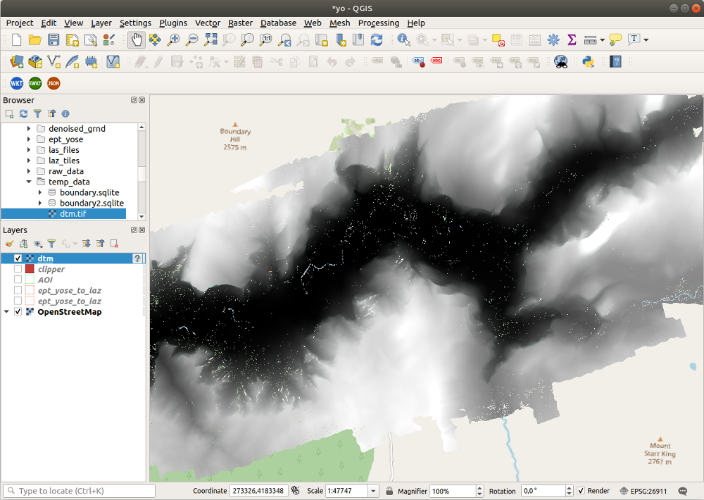
zoomed
Generate a Hillshade from the DTM (Digital Terrain Model).
gdaldem hillshade temp_data/dtm.tif \
    temp_data/hillshade.tif \
    -z 1.0 -s 1.0 -az 315.0 -alt 45.0 \
    -of GTiff
(new_clouds) myuser@comp:~/yose$ gdaldem hillshade temp_data/dtm.tif \
> temp_data/hillshade.tif \
> -z 1.0 -s 1.0 -az 315.0 -alt 45.0 \
> -of GTiff
0...10...20...30...40...50...60...70...80...90...100 - done.
(new_clouds) myuser@comp:~/yose$
hillshade in qgis 
zoomed
Creating surface meshes (src)
TODO
Rasterizing Attributes (src)
Generate a raster surface using a fully classified point cloud. Create a file named classification.json and populate it with the below code, then run pdal pipeline.
{
    "pipeline":[
        {
            "type":"readers.las",
            "filename":"temp_data/ept_yose_to_laz.laz"
        },
        {
            "type":"writers.gdal",
            "filename":"temp_data/yose-classification.tif",
            "dimension":"Classification",
            "data_type":"uint16_t",
            "output_type":"mean",
            "resolution": 1
        }
    ]
}
pdal pipeline classification.json -v 3
tree temp_data/(new_clouds) myuser@comp:~/yose$ pdal pipeline classification.json -v 3
(PDAL Debug) Debugging...
(pdal pipeline Debug) Executing pipeline in stream mode.
(new_clouds) myuser@comp:~/yose$ tree temp_data/
temp_data/
├── boundary2.sqlite
├── boundary.sqlite
├── clean.laz
├── denoised_ground.laz
├── dtm.tif
├── ept_yose_to_laz.laz
├── hillshade.tif
├── points_little_yose_wgs84.laz
├── thin.laz
└── yose-classification.tif
0 directories, 11 files
(new_clouds) myuser@comp:~/yose$
Classification in qgis 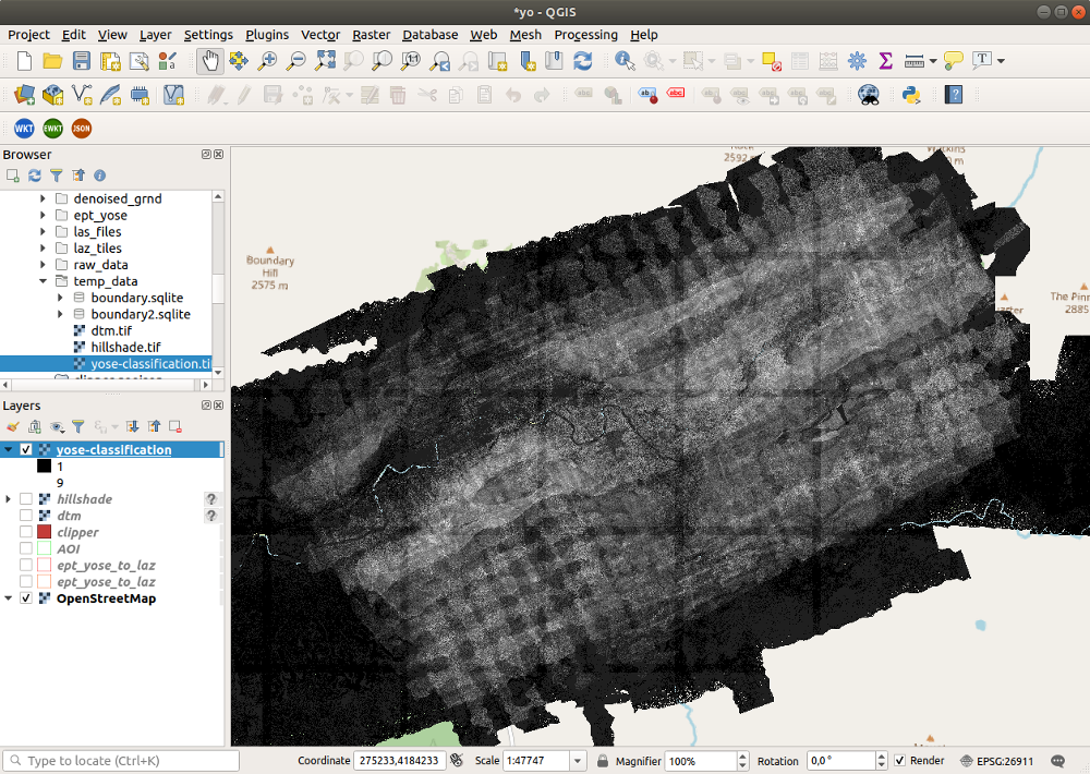
zoomed
Then create a file named colours.txt and enter the code below, that gdaldem can consume to apply colors to the data, and QGIS can use as color map.
# QGIS Generated Color Map Export File
2 139 51 38 255 Ground
3 143 201 157 255 Low Veg
4 5 159 43 255 Med Veg
5 47 250 11 255 High Veg
6 209 151 25 255 Building
7 232 41 7 255 Low Point
8 197 0 204 255 reserved
9 26 44 240 255 Water
10 165 160 173 255 Rail
11 81 87 81 255 Road
12 203 210 73 255 Reserved
13 209 228 214 255 Wire - Guard (Shield)
14 160 168 231 255 Wire - Conductor (Phase)
15 220 213 164 255 Transmission Tower
16 214 211 143 255 Wire-Structure Connector (Insulator)
17 151 98 203 255 Bridge Deck
18 236 49 74 255 High Noise
19 185 103 45 255 Reserved
21 58 55 9 255 255 Reserved
22 76 46 58 255 255 Reserved
23 20 76 38 255 255 Reserved
26 78 92 32 255 255 Reserved
gdaldem color-relief temp_data/yose-classification.tif colours.txt temp_data/classified-color.png -of PNG(new_clouds) myuser@comp:~/yose$ gdaldem color-relief temp_data/yose-classification.tif colours.txt temp_data/classified-color.png -of PNG
0...10...20...30...40...50...60...70...80...90...100 - done.
(new_clouds) myuser@comp:~/yose$
classified color in qgis 
zoomed
Then generate a relative intensity image.
pdal pipeline classification.json \
    --writers.gdal.dimension="Intensity" \
    --writers.gdal.data_type="float" \
    --writers.gdal.filename="temp_data/intensity.tif" \
    -v 3
(new_clouds) myuser@comp:~/yose$ pdal pipeline classification.json \
> --writers.gdal.dimension="Intensity" \
> --writers.gdal.data_type="float" \
> --writers.gdal.filename="temp_data/intensity.tif" \
> -v 3
(PDAL Debug) Debugging...
(pdal pipeline Debug) Executing pipeline in stream mode.
(new_clouds) myuser@comp:~/yose$gdal_translate temp_data/intensity.tif temp_data/intensity.png -of PNG(new_clouds) myuser@comp:~/yose$ gdal_translate temp_data/intensity.tif temp_data/intensity.png -of PNG
Input file size is 22747, 9618
Warning 6: PNG driver doesn't support data type Float32. Only eight bit (Byte) and sixteen bit (UInt16) bands supported. Defaulting to Byte
0...10...20...30...40...50...60...70...80...90...100 - done.
(new_clouds) myuser@comp:~/yose$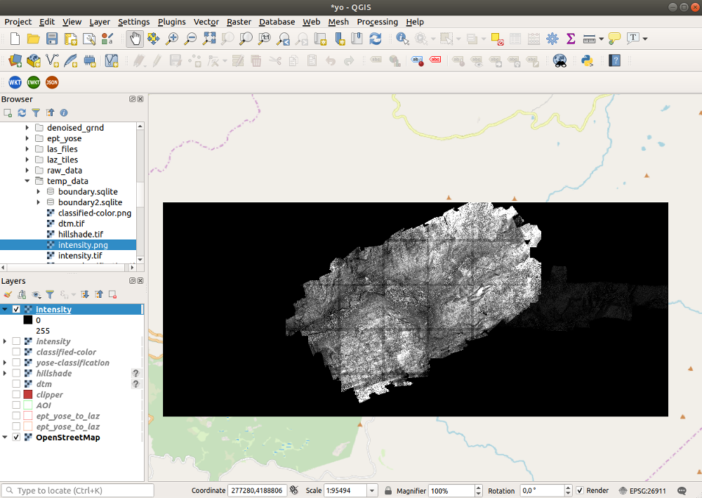
intensity in qgis 
zoomed
Plotting a histogram using Python (src)
TODO: killed. The image above is from the Taal Volcano experiments.
{
    "pipeline": [
        {
            "filename": "temp_data/ept_yose_to_laz.laz"
        },
        {
            "type": "filters.python",
            "function": "make_plot",
            "module": "anything",
            "pdalargs": "{\"filename\":\"temp_data/histogram.png\"}",
            "script": "histogram.py"
        },
        {
            "type": "writers.null"
        }
    ]
}
# import numpy
import numpy as np
# import matplotlib stuff and make sure to use the
# AGG renderer.
import matplotlib
matplotlib.use('Agg')
import matplotlib.pyplot as plt
import matplotlib.mlab as mlab
# This only works for Python 3. Use
# StringIO for Python 2.
from io import BytesIO
# The make_plot function will do all of our work. The
# filters.programmable filter expects a function name in the
# module that has at least two arguments -- "ins" which
# are numpy arrays for each dimension, and the "outs" which
# the script can alter/set/adjust to have them updated for
# further processing.
def make_plot(ins, outs):
# figure position and row will increment
figure_position = 1
row = 1
fig = plt.figure(figure_position, figsize=(6, 8.5), dpi=300)
for key in ins:
dimension = ins[key]
ax = fig.add_subplot(len(ins.keys()), 1, row)
# histogram the current dimension with 30 bins
n, bins, patches = ax.hist( dimension, 30,
facecolor='grey',
alpha=0.75,
align='mid',
histtype='stepfilled',
linewidth=None)
# Set plot particulars
ax.set_ylabel(key, size=10, rotation='horizontal')
ax.get_xaxis().set_visible(False)
ax.set_yticklabels('')
ax.set_yticks((),)
ax.set_xlim(min(dimension), max(dimension))
ax.set_ylim(min(n), max(n))
# increment plot position
row = row + 1
figure_position = figure_position + 1
# We will save the PNG bytes to a BytesIO instance
# and the nwrite that to a file.
output = BytesIO()
plt.savefig(output,format="PNG")
# a module global variable, called 'pdalargs' is available
# to filters.programmable and filters.predicate modules that contains
# a dictionary of arguments that can be explicitly passed into
# the module by the user. We passed in a filename arg in our `pdal pipeline` call
if 'filename' in pdalargs:
filename = pdalargs['filename']
else:
filename = 'histogram.png'
# open up the filename and write out the
# bytes of the PNG stored in the BytesIO instance
o = open(filename, 'wb')
o.write(output.getvalue())
o.close()
# filters.programmable scripts need to
# return True to tell the filter it was successful.
return Truepython -m pip install -U matplotlib==3.2.0rc1
pdal pipeline histogram.json(new_clouds) myuser@comp:~/yose$ pdal pipeline histogram.json
anything:46: UserWarning: Attempting to set identical left == right == 0 results in singular transformations; automatically expanding.
(new_clouds) myuser@comp:~/yose$
Python histogram for laz file
Batch Processing (src)
Example syntax. There is another example in Identifying ground section.
# Create directory unless exists
mkdir -pv gtiles
# List files in Windows dos and iterate them
# use verbose to view logs
for %f in (*.*) do pdal pipeline denoise_ground.json ^
   --readers.las.filename=%f ^
   --writers.las.filename=../gtiles/%f
   --verbose 4

# Create directory unless exists
mkdir -pv denoised_grnd
# List files in Linux shell and iterate them
ls laz_tiles/*.laz | \
parallel -I{} pdal pipeline denoise_ground.json \
    --readers.las.filename={} \
    --writers.las.filename=denoised_grnd/denoised_grnd{/.}.laz \
    --verbose 4
✅ Repeated the steps for Yosemite Valley
What’s next?
☑️ Repeat the steps for an urban area
☑️ Then try LasTools, too
☑️ And, of course, the 3D in Blender. 😀
PS: You can admire each dataset directly in Potree using Generate 3D point cloud browser visualization on OpenTopography corresponding page.
Reminder: The colored point cloud data that we have used throughout this post can be viewed at https://potree.entwine.io/data/view.html?r=”https://maptheclouds.com/ept_yose_colored/”.
Below, I leave you a Potree mix of all the Yosemite Valley, from my personal computer.

Yosemite Valley 
The Dome 
El Capitan