
Those are my notes on taking some LiDAR data and testing different commands in PDAL. If you like, you can follow along using your own data.
Probably I’ll de adding or deleting stuff, but you can take a look to see some of the main operations that can be made on point clouds using PDAL.
This is an adaptation of the original workshop from the PDAL website, Point Cloud Processing and Analysis with PDAL, the single difference being that I use the same data for every operation and show the commands output, too, while in the workshop there are used different data sources.
The workshop can be downloaded from here, too.
The point cloud data that we will be using throughout this post can be viewed here: https://potree.entwine.io/data/view.html?r=”https://phil-lidar-taal-entwine-s3.s3.us-east-2.amazonaws.com/Taal_Volcano_Island/”.
You can use Fugro Viewer or LASTools to view LiDAR files on desktop, but only in Windows! The Linux users, although forgotten, are lucky to have Potree and Plasio that can consume Entwine Point Tile (EPT) datasets in the browser. But let’s just approach LiDAR with baby steps before digging too deep. 🙂
LiDAR is a remote sensing technique that uses visible or near-infrared laser energy to measure the distance between a sensor and an object. The sensors can be terrestrial (on tripod), airborne (plane), mobile (car) and unmanned (drones).
PDAL, Point Data Abstraction Library, is a C/C++ open source library and applications for translating and processing point cloud data.
I won’t go into details about LiDAR, feel free to read this comprehensive guide: Lidar 101: An Introduction to Lidar Technology, Data, and Applications.
Download the data
You can use your own files, but I’ll be using free data for the Philippines Taal Vulcano. This volcano has a sad story, it has recently errupted, in January.
I have downloaded LiDAR files in the compressed LAZ format, from Taal Open LiDAR, after I found out about it on rapidlasso GmbH. The data was collected for the UP TCAGP and PHIL-LiDAR Program (details). There are multiple 1 meter LAZ tiles that each cover an area of 1000 by 1000 meter:
.
└── raw_data
    ├── E280N1553_LAZ_PL1.laz
    ├── E281N1547_LAZ_PL1.laz
    ├── E281N1548_LAZ_PL1.laz
    ├── E281N1549_LAZ_PL1.laz
    ├── E281N1550_LAZ_PL1.laz
    ├── E281N1551_LAZ_PL1.laz
    ├── E281N1552_LAZ_PL1.laz
    ├── E281N1553_LAZ_PL1.laz
    ├── E282N1547_LAZ_PL1.laz
    ├── E282N1548_LAZ_PL1.laz
    ├── E282N1549_LAZ_PL1.laz
    ├── E282N1550_LAZ_PL1.laz
    ├── E282N1551_LAZ_PL1.laz
    ├── E282N1552_LAZ_PL1.laz
    ├── E282N1553_LAZ_PL1.laz
    ├── E283N1548_LAZ_PL1.laz
    ├── E283N1549_LAZ_PL1.laz
    ├── E283N1550_LAZ_PL1.laz
    ├── E283N1551_LAZ_PL1.laz
    ├── E283N1552_LAZ_PL1.laz
    ├── E283N1553_LAZ_PL1.laz
    ├── E284N1548_LAZ_PL1.laz
    ├── E284N1549_LAZ_PL1.laz
    ├── E284N1550_LAZ_PL1.laz
    ├── E284N1551_LAZ_PL1.laz
    ├── E284N1552_LAZ_PL1.laz
    ├── E284N1553_LAZ_PL1.laz
    ├── E285N1548_LAZ_PL1.laz
    ├── E285N1549_LAZ_PL1.laz
    ├── E285N1550_LAZ_PL1.laz
    ├── E285N1551_LAZ_PL1.laz
    ├── E285N1552_LAZ_PL1.laz
    ├── E285N1553_LAZ_PL1.laz
    ├── E285N1554_LAZ_PL1.laz
    └── E286N1551_LAZ_PL1.laz

LiPAD download portal 
LiPAD – TAAL VOLCANO
Alternatively, you can use data from OpenTopography, like this portion of Yosemite Valley that I have used in another post. Keep in mind that if the dataset is too large, you should split it in tiles before working with it. For example, for Yosemite I’ve used:
pdal tile processed_files/yosemite_merged.laz "tiles/yose_#.laz"We create a working folder, phili and a subfolder named raw_data, then move all the downloaded point cloud data into it.
# go home, create subdirectory and parent directory
cd && mkdir -pv phili/raw_data
Install PDAL
You can read this other post to find out how to install PDAL. Every time you want to access the environment where PDAL was installed, useconda activate followed by the environment name, in our case new_clouds.
I will refer to Linux, though the commands for Windows will be mentioned, too. NOTE: PDAL commands, except batch processing, are the same in Windows and Linux, but the line separator differs: ^ in Windows and \ in Linux.
Play
Printing the first point (src)
# List the LAZ files
cd ~/phili
ls -lah raw_data
# Query the las data using pdal info
pdal info raw_data/E280N1553_LAZ_PL1.laz -p 0
(new_clouds) myuser@comp:~/phili$ pdal info raw_data/E280N1553_LAZ_PL1.laz -p 0
{
"filename": "raw_data/E280N1553_LAZ_PL1.laz",
"pdal_version": "2.0.1 (git-version: 6600e6)",
"points":
{
"point":
{
"Classification": 1,
"EdgeOfFlightLine": 0,
"GpsTime": 270635.4339,
"Intensity": 15,
"NumberOfReturns": 1,
"PointId": 0,
"PointSourceId": 1010,
"ReturnNumber": 1,
"ScanAngleRank": -26,
"ScanDirectionFlag": 0,
"UserData": 0,
"X": 280999.99,
"Y": 1552622.08,
"Z": 260.8
}
}
}Printing file metadata (src)
pdal info raw_data/E280N1553_LAZ_PL1.laz --metadata(new_clouds) myuser@comp:~/phili$ pdal info raw_data/E280N1553_LAZ_PL1.laz --metadata
{
"filename": "raw_data/E280N1553_LAZ_PL1.laz",
"metadata":
{
"comp_spatialreference": "",
"compressed": true,
"count": 902276,
"creation_doy": 46,
"creation_year": 2016,
"dataformat_id": 1,
"dataoffset": 329,
"filesource_id": 0,
"global_encoding": 0,
"global_encoding_base64": "AAA=",
"header_size": 227,
"major_version": 1,
"maxx": 280999.99,
"maxy": 1552669.86,
"maxz": 262.28,
"minor_version": 2,
"minx": 280427.5,
"miny": 1552000,
"minz": 46.3,
"offset_x": 0,
"offset_y": 0,
"offset_z": 0,
"point_length": 28,
"project_id": "00000000-0000-0000-0000-000000000000",
"scale_x": 0.01,
"scale_y": 0.01,
"scale_z": 0.01,
"software_id": "TerraScan",
"spatialreference": "",
"srs":
{
"compoundwkt": "",
"horizontal": "",
"isgeocentric": false,
"isgeographic": false,
"prettycompoundwkt": "",
"prettywkt": "",
"proj4": "",
"units":
{
"horizontal": "unknown",
"vertical": ""
},
"vertical": "",
"wkt": ""
},
"system_id": "",
"vlr_0":
{
"data": "AgAAAAICAAAAAAAAUMMAAP////////////////////8CAAYAFAACAAcACAACAA==",
"description": "by laszip of LAStools (150202)",
"record_id": 22204,
"user_id": "laszip encoded"
}
},
"pdal_version": "2.0.1 (git-version: 6600e6)"
}Install jq with sudo apt install jq (on Windows from https://stedolan.github.io/jq), then filter the JSON query result using jq.
(new_clouds) myuser@comp:~/phili$ pdal info raw_data/E280N1553_LAZ_PL1.laz --metadata | jq  ".metadata.maxx, .metadata.count"
280999.99
902276
Find the midpoint of the bounding cube (src)
(new_clouds) myuser@comp:~/phili$ pdal info raw_data/E280N1553_LAZ_PL1.laz --all | jq .stats.bbox.native.bbox
{
  "maxx": 280999.99,
  "maxy": 1552669.86,
  "maxz": 262.28,
  "minx": 280427.5,
  "miny": 1552000,
  "minz": 46.3
}
Calculate the average the X, Y, and Z values for this tile: min + (max – min)/2
- x = 280427.5 + (280999.99 – 280427.5)/2 = 280713.745
- y = 1552000 + (1552669.86 – 1552000)/2 = 1552334.930
- z = 46.3 + (262.28 – 46.3)/2 = 154.290
(new_clouds) myuser@comp:~/phili$ python
Python 3.8.1 | packaged by conda-forge | (default, Jan 29 2020, 14:55:04)
[GCC 7.3.0] on linux
Type "help", "copyright", "credits" or "license" for more information.
>>> 280427.5 + (280999.99 - 280427.5)/2
280713.745
>>> 1552000 + (1552669.86 - 1552000)/2
1552334.9300000002
>>> 46.3 + (262.28 - 46.3)/2
154.28999999999996
>>> exit()
(new_clouds) myuser@comp:~/phili$
Now we can return the three nearest points from the calculated center.
(new_clouds) myuser@comp:~/phili$ pdal info raw_data/E280N1553_LAZ_PL1.laz --query "280713.745, 1552334.930, 154.290/3"
{
  "filename": "raw_data/E280N1553_LAZ_PL1.laz",
  "pdal_version": "2.0.1 (git-version: 6600e6)",
  "points":
  {
    "point":
    [
      {
        "Classification": 1,
        "EdgeOfFlightLine": 0,
        "GpsTime": 270635.4342,
        "Intensity": 9,
        "NumberOfReturns": 1,
        "PointId": 42,
        "PointSourceId": 1010,
        "ReturnNumber": 1,
        "ScanAngleRank": -26,
        "ScanDirectionFlag": 1,
        "UserData": 0,
        "X": 280999.98,
        "Y": 1552622.09,
        "Z": 262.28
      },
      {
        "Classification": 1,
        "EdgeOfFlightLine": 0,
        "GpsTime": 270635.434,
        "Intensity": 16,
        "NumberOfReturns": 1,
        "PointId": 19,
        "PointSourceId": 1010,
        "ReturnNumber": 1,
        "ScanAngleRank": -26,
        "ScanDirectionFlag": 0,
        "UserData": 0,
        "X": 280999.91,
        "Y": 1552622.26,
        "Z": 262.15
      },
      {
        "Classification": 1,
        "EdgeOfFlightLine": 0,
        "GpsTime": 270635.4341,
        "Intensity": 14,
        "NumberOfReturns": 1,
        "PointId": 34,
        "PointSourceId": 1010,
        "ReturnNumber": 1,
        "ScanAngleRank": -26,
        "ScanDirectionFlag": 1,
        "UserData": 0,
        "X": 280999.89,
        "Y": 1552622.3,
        "Z": 262.13
      }
    ]
  }
}
(new_clouds) myuser@comp:~/phili$
Compression and Decompression (src)
Create a new folder named temp_data, decompress the file from LAZ to LAS using pdal translate, then compare their size.
(new_clouds) myuser@comp:~/phili$ mkdir temp_data && pdal translate raw_data/E280N1553_LAZ_PL1.laz temp_data/E280N1553_LAZ_PL1.las
(new_clouds) myuser@comp:~/phili$ ls -lah raw_data/E280N1553_LAZ_PL1.laz
-rwxrwxrwx 1 myuser myuser 3,1M feb  6 20:52 raw_data/E280N1553_LAZ_PL1.laz
(new_clouds) myuser@comp:~/phili$ ls -lah temp_data/E280N1553_LAZ_PL1.las
-rw-r--r-- 1 myuser myuser 30M feb  7 00:17 temp_data/E280N1553_LAZ_PL1.las
(new_clouds) myuser@comp:~/phili$
Reprojection (src)
Reproject file using pdal translate. There was no information about the coordinate system in the LAZ file, I had to download a DTM from the website to find out it was “EPSG:32651”.
pdal translate raw_data/E280N1553_LAZ_PL1.laz \
    temp_data/E280N1553_LAZ_PL1_WGS.laz reprojection \
    --filters.reprojection.in_srs="EPSG:32651" \
    --filters.reprojection.out_srs="EPSG:4326"
pdal info temp_data/E280N1553_LAZ_PL1_WGS.laz --all | jq .stats.bbox.native.bbox
pdal info temp_data/E280N1553_LAZ_PL1_WGS.laz -p 0
(new_clouds) myuser@comp:~/phili$ pdal translate raw_data/E280N1553_LAZ_PL1.laz \
> temp_data/E280N1553_LAZ_PL1_WGS.laz reprojection \
> --filters.reprojection.in_srs="EPSG:32651" \
> --filters.reprojection.out_srs="EPSG:4326"
(new_clouds) myuser@comp:~/phili$ pdal info temp_data/E280N1553_LAZ_PL1_WGS.laz --all | jq .stats.bbox.native.bbox
{
"maxx": 120.97,
"maxy": 14.04,
"maxz": 262.28,
"minx": 120.97,
"miny": 14.03,
"minz": 46.3
}
(new_clouds) myuser@comp:~/phili$ pdal info temp_data/E280N1553_LAZ_PL1_WGS.laz -p 0
{
"filename": "temp_data/E280N1553_LAZ_PL1_WGS.laz",
"pdal_version": "2.0.1 (git-version: 6600e6)",
"points":
{
"point":
{
"Blue": 0,
"Classification": 1,
"EdgeOfFlightLine": 0,
"GpsTime": 270635.4339,
"Green": 0,
"Intensity": 15,
"NumberOfReturns": 1,
"PointId": 0,
"PointSourceId": 1010,
"Red": 0,
"ReturnNumber": 1,
"ScanAngleRank": -26,
"ScanDirectionFlag": 0,
"UserData": 0,
"X": 120.97,
"Y": 14.04,
"Z": 260.8
}
}
}
(new_clouds) myuser@comp:~/phili$For latitude/longitude data, you will need to set the scale to smaller values like 0.0000001. Repeat the reproject command setting the scale, too.
pdal translate raw_data/E280N1553_LAZ_PL1.laz \
    temp_data/E280N1553_LAZ_PL1_WGS.laz reprojection \
    --filters.reprojection.in_srs="EPSG:32651" \
    --filters.reprojection.out_srs="EPSG:4326" \
    --writers.las.scale_x=0.0000001 \
    --writers.las.scale_y=0.0000001 \
    --writers.las.offset_x="auto" \
    --writers.las.offset_y="auto"
pdal info temp_data/E280N1553_LAZ_PL1_WGS.laz --all | jq .stats.bbox.native.bbox
pdal info temp_data/E280N1553_LAZ_PL1_WGS.laz -p 0
(new_clouds) myuser@comp:~/phili$ pdal translate raw_data/E280N1553_LAZ_PL1.laz \
> temp_data/E280N1553_LAZ_PL1_WGS.laz reprojection \
> --filters.reprojection.in_srs="EPSG:32651" \
> --filters.reprojection.out_srs="EPSG:4326" \
> --writers.las.scale_x=0.0000001 \
> --writers.las.scale_y=0.0000001 \
> --writers.las.offset_x="auto" \
> --writers.las.offset_y="auto"
(pdal translate writers.las Warning) Auto offset for Xrequested in stream mode. Using value of 120.972.
(pdal translate writers.las Warning) Auto offset for Yrequested in stream mode. Using value of 14.0358.
(new_clouds) myuser@comp:~/phili$ pdal info temp_data/E280N1553_LAZ_PL1_WGS.laz --all | jq .stats.bbox.native.bbox
{
"maxx": 120.9721603,
"maxy": 14.03619005,
"maxz": 262.28,
"minx": 120.9668247,
"miny": 14.03012035,
"minz": 46.3
}
(new_clouds) myuser@comp:~/phili$ pdal info temp_data/E280N1553_LAZ_PL1_WGS.laz -p 0
{
"filename": "temp_data/E280N1553_LAZ_PL1_WGS.laz",
"pdal_version": "2.0.1 (git-version: 6600e6)",
"points":
{
"point":
{
"Blue": 0,
"Classification": 1,
"EdgeOfFlightLine": 0,
"GpsTime": 270635.4339,
"Green": 0,
"Intensity": 15,
"NumberOfReturns": 1,
"PointId": 0,
"PointSourceId": 1010,
"Red": 0,
"ReturnNumber": 1,
"ScanAngleRank": -26,
"ScanDirectionFlag": 0,
"UserData": 0,
"X": 120.9721111,
"Y": 14.03576605,
"Z": 260.8
}
}
}
(new_clouds) myuser@comp:~/phili$Entwine (src)
We will use Entwine to create a new folder named ept_phili, then rearrange points into a lossless octree structure known as EPT.
You can read this other post to find out how to install Entwine.
The build command is used to generate an Entwine Point Tile (EPT) dataset from point cloud data. Because we want to build the visualization from all of our data, for input we provide the path to raw_data folder the command.
entwine build -i raw_data/*.laz -o ept_phili --srs "EPSG:32651"(new_clouds) myuser@comp:~/phili$ entwine build -i raw_data/*.laz -o ept_phili --srs "EPSG:32651"
Scanning input
1/35: raw_data/E280N1553_LAZ_PL1.laz
2/35: raw_data/E281N1547_LAZ_PL1.laz
3/35: raw_data/E281N1548_LAZ_PL1.laz
4/35: raw_data/E281N1549_LAZ_PL1.laz
5/35: raw_data/E281N1550_LAZ_PL1.laz
6/35: raw_data/E281N1551_LAZ_PL1.laz
7/35: raw_data/E281N1552_LAZ_PL1.laz
8/35: raw_data/E281N1553_LAZ_PL1.laz
9/35: raw_data/E282N1547_LAZ_PL1.laz
10/35: raw_data/E282N1548_LAZ_PL1.laz
11/35: raw_data/E282N1549_LAZ_PL1.laz
12/35: raw_data/E282N1550_LAZ_PL1.laz
13/35: raw_data/E282N1551_LAZ_PL1.laz
14/35: raw_data/E282N1552_LAZ_PL1.laz
15/35: raw_data/E282N1553_LAZ_PL1.laz
16/35: raw_data/E283N1548_LAZ_PL1.laz
17/35: raw_data/E283N1549_LAZ_PL1.laz
18/35: raw_data/E283N1550_LAZ_PL1.laz
19/35: raw_data/E283N1551_LAZ_PL1.laz
20/35: raw_data/E283N1552_LAZ_PL1.laz
21/35: raw_data/E283N1553_LAZ_PL1.laz
22/35: raw_data/E284N1548_LAZ_PL1.laz
23/35: raw_data/E284N1549_LAZ_PL1.laz
24/35: raw_data/E284N1550_LAZ_PL1.laz
25/35: raw_data/E284N1551_LAZ_PL1.laz
26/35: raw_data/E284N1552_LAZ_PL1.laz
27/35: raw_data/E284N1553_LAZ_PL1.laz
28/35: raw_data/E285N1548_LAZ_PL1.laz
29/35: raw_data/E285N1549_LAZ_PL1.laz
30/35: raw_data/E285N1550_LAZ_PL1.laz
31/35: raw_data/E285N1551_LAZ_PL1.laz
32/35: raw_data/E285N1552_LAZ_PL1.laz
33/35: raw_data/E285N1553_LAZ_PL1.laz
34/35: raw_data/E285N1554_LAZ_PL1.laz
35/35: raw_data/E286N1551_LAZ_PL1.laz
Entwine Version: 2.1.0
EPT Version: 1.0.0
Input:
Files: 35
Total points: 172,148,957
Density estimate (per square unit): 5.43294
Threads: [3, 5]
Output:
Path: ept_phili/
Data type: laszip
Hierarchy type: json
Sleep count: 2,097,152
Scale: 0.01
Offset: (283714, 1550170, 120)
Metadata:
SRS: EPSG:32651
Bounds: [(280427, 1546340, -140), (287000, 1554000, 380)]
Cube: [(279883, 1546339, -3711), (287545, 1554001, 3951)]
Storing dimensions: [
X:int32, Y:int32, Z:int32, Intensity:uint16, ReturnNumber:uint8,
NumberOfReturns:uint8, ScanDirectionFlag:uint8,
EdgeOfFlightLine:uint8, Classification:uint8, ScanAngleRank:float,
UserData:uint8, PointSourceId:uint16, GpsTime:double, OriginId:uint32
]
Build parameters:
Span: 128
Resolution 2D: 128 * 128 = 16,384
Resolution 3D: 128 * 128 * 128 = 2,097,152
Maximum node size: 65,536
Minimum node size: 16,384
Cache size: 64
Adding 0 - raw_data/E280N1553_LAZ_PL1.laz
Adding 1 - raw_data/E281N1547_LAZ_PL1.laz
Adding 2 - raw_data/E281N1548_LAZ_PL1.laz
Adding 3 - raw_data/E281N1549_LAZ_PL1.laz
Adding 4 - raw_data/E281N1550_LAZ_PL1.laz
Done 0
Adding 5 - raw_data/E281N1551_LAZ_PL1.laz
Done 1
Adding 6 - raw_data/E281N1552_LAZ_PL1.laz
Done 2
Adding 7 - raw_data/E281N1553_LAZ_PL1.laz
00:10 - 10% - 16,730,384 - 6,022(6,022)M/h - 122W - 5R - 334A
Done 3
Adding 8 - raw_data/E282N1547_LAZ_PL1.laz
Done 4
Adding 9 - raw_data/E282N1548_LAZ_PL1.laz
00:20 - 19% - 32,115,196 - 5,780(5,538)M/h - 409W - 28R - 369A
Done 5
Adding 10 - raw_data/E282N1549_LAZ_PL1.laz
Done 8
Adding 11 - raw_data/E282N1550_LAZ_PL1.laz
Done 6
Adding 12 - raw_data/E282N1551_LAZ_PL1.laz
Done 7
Adding 13 - raw_data/E282N1552_LAZ_PL1.laz
00:30 - 26% - 45,330,267 - 5,439(4,757)M/h - 437W - 60R - 335A
Done 9
Adding 14 - raw_data/E282N1553_LAZ_PL1.laz
00:40 - 34% - 59,255,561 - 5,333(5,013)M/h - 435W - 72R - 351A
Done 10
Adding 15 - raw_data/E283N1548_LAZ_PL1.laz
Done 11
Adding 16 - raw_data/E283N1549_LAZ_PL1.laz
Done 14
Adding 17 - raw_data/E283N1550_LAZ_PL1.laz
00:50 - 43% - 73,172,066 - 5,268(5,009)M/h - 375W - 54R - 383A
Done 12
Adding 18 - raw_data/E283N1551_LAZ_PL1.laz
Done 15
Adding 19 - raw_data/E283N1552_LAZ_PL1.laz
Done 13
Adding 20 - raw_data/E283N1553_LAZ_PL1.laz
01:00 - 50% - 86,871,954 - 5,212(4,931)M/h - 519W - 64R - 267A
Done 17
Adding 21 - raw_data/E284N1548_LAZ_PL1.laz
Done 16
Adding 22 - raw_data/E284N1549_LAZ_PL1.laz
01:10 - 59% - 101,289,352 - 5,209(5,190)M/h - 395W - 41R - 286A
Done 18
Adding 23 - raw_data/E284N1550_LAZ_PL1.laz
Done 21
Adding 24 - raw_data/E284N1551_LAZ_PL1.laz
Done 20
Adding 25 - raw_data/E284N1552_LAZ_PL1.laz
Done 19
Adding 26 - raw_data/E284N1553_LAZ_PL1.laz
01:20 - 67% - 115,187,943 - 5,183(5,003)M/h - 448W - 71R - 265A
Done 23
Adding 27 - raw_data/E285N1548_LAZ_PL1.laz
Done 22
Adding 28 - raw_data/E285N1549_LAZ_PL1.laz
01:30 - 75% - 129,260,740 - 5,170(5,066)M/h - 489W - 69R - 245A
Done 24
Adding 29 - raw_data/E285N1550_LAZ_PL1.laz
Done 27
Adding 30 - raw_data/E285N1551_LAZ_PL1.laz
Done 26
Adding 31 - raw_data/E285N1552_LAZ_PL1.laz
01:40 - 84% - 143,799,941 - 5,176(5,234)M/h - 356W - 68R - 335A
Done 28
Adding 32 - raw_data/E285N1553_LAZ_PL1.laz
Done 25
Adding 33 - raw_data/E285N1554_LAZ_PL1.laz
Done 29
Adding 34 - raw_data/E286N1551_LAZ_PL1.laz
01:50 - 92% - 157,579,245 - 5,157(4,960)M/h - 454W - 58R - 310A
Done 30
Pushes complete - joining...
Done 31
02:00 - 99% - 170,642,287 - 5,119(4,702)M/h - 437W - 71R - 237A
Done 34
Done 32
Done 33
Reawakened: 661
Saving registry...
Saving metadata...
Index completed in 02:04.
Save complete.
Points inserted: 172,148,957
(new_clouds) myuser@comp:~/phili$(new_clouds) myuser@comp:~/phili$ tree ept_phili/
ept_phili/
├── ept-build.json
├── ept-data
│ ├── 0-0-0-0.laz
│ ├── 1-0-0-0.laz
│ ├── 1-0-0-1.laz
│ ├── 1-0-1-0.laz
│ ├── 1-0-1-1.laz
│ ├── 1-1-0-0.laz
[...]
│ ├── 7-99-70-63.laz
│ ├── 7-99-71-63.laz
│ ├── 7-99-72-63.laz
│ └── 7-99-75-63.laz
├── ept-hierarchy
│ └── 0-0-0-0.json
├── ept.json
└── ept-sources
├── 0.json
└── list.json
3 directories, 4489 files
(new_clouds) myuser@comp:~/phili$Now we can statically serve the entwine directory with an HTTP server and visualize it with the WebGL-based Potree and Plasio projects.
Potree and Plasio
We can visualize our data in Potree and Plasio, directly in the browser.
# Install NodeJS and http server from nodejs
conda install nodejs -y
npm install http-server -g
# Make sure you are in the working folder, and the EPT folder
# is a subfolder
# Start the server using --cors to allow serving data to the
# remote Potree/Plasio pages
http-server -p 8066 --cors
(new_clouds) myuser@comp:~/phili$ http-server -p 8066 --cors
Starting up http-server, serving ./
Available on:
http://127.0.0.1:8066
http://192.168.0.102:8066
http://172.18.0.1:8066
http://192.168.61.1:8066
http://192.168.63.1:8066
Hit CTRL-C to stop the server# In another tab (Shift+Ctrl+T), visualise out local point cloud data in Potree
xdg-open "http://potree.entwine.io/data/view.html?r=http://localhost:8066/ept_phili"Assign a colour scale to the points based on elevation, classification and other criteria, then play with some terrain profiles.
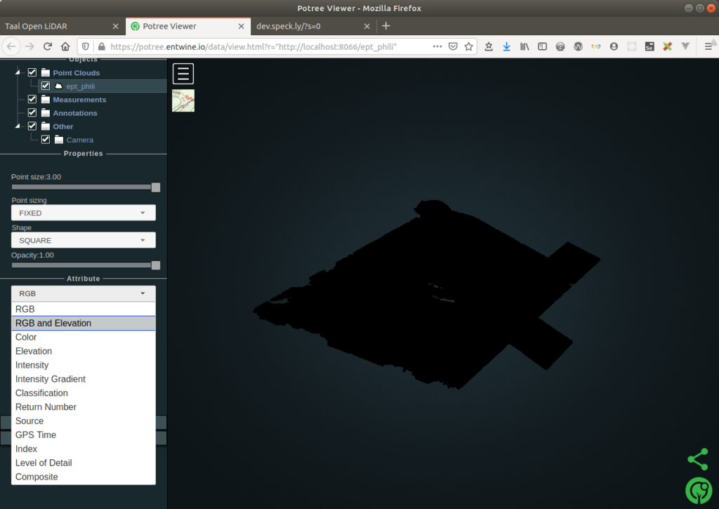
First view 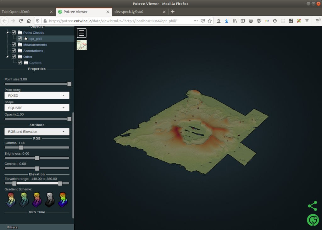
color by elevation 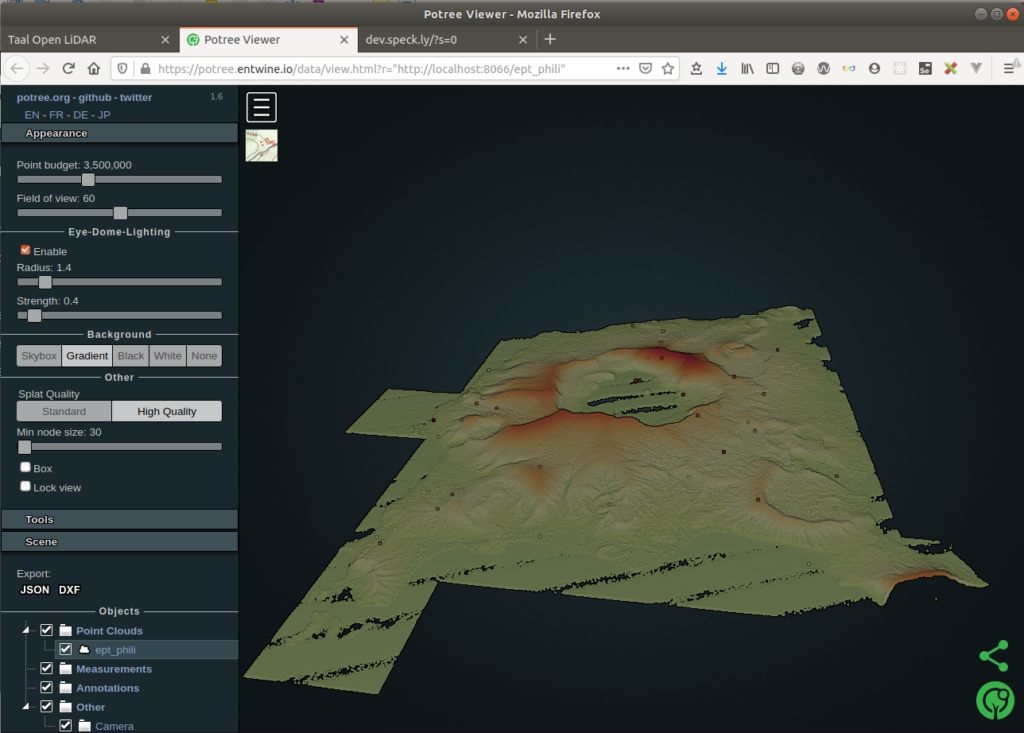
zoom 
zoom 
profile highlight 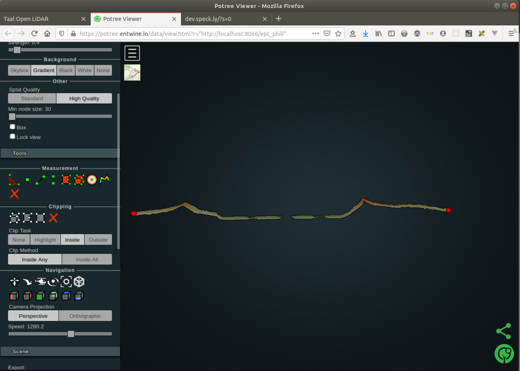
profile inside 
profile highlight 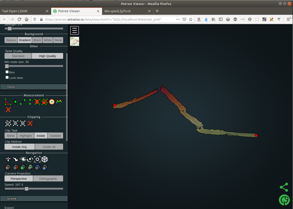
profile inside 
profile highlight 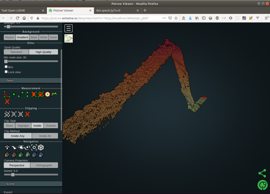
profile inside 
profile outside 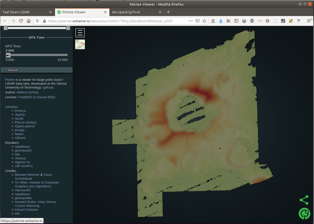
potree about


Visualize the points by elevation:

BY ELEVATION 
hide high vegetation 
hide medium vegetation 
hide low vegetation 
BY ELEVATION 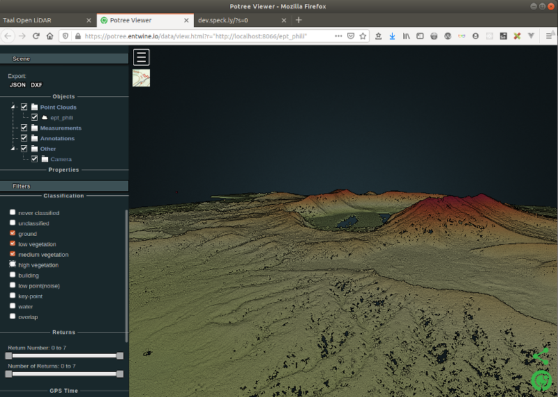
hide high vegetation 
hide medium vegetation 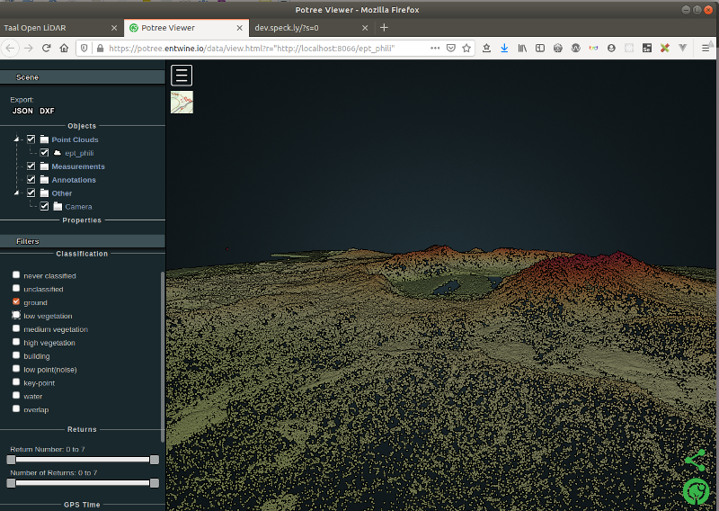
hide low vegetation
Visualize the points by point classification:

ground 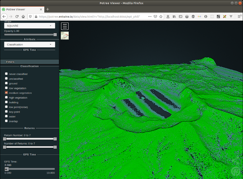
medium vegetation 
high vegetation 
noise 
key point 
All 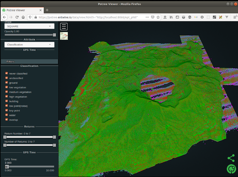
all 
all – trees
Visualize the points in Plasio, too.
# Visualise our local point cloud data in Plasio

xdg-open "http://dev.speck.ly/?s=0&r=ept://localhost:8066/ept_phili&c0s=local://color"
First view 
color by elevation 
satellite imagery 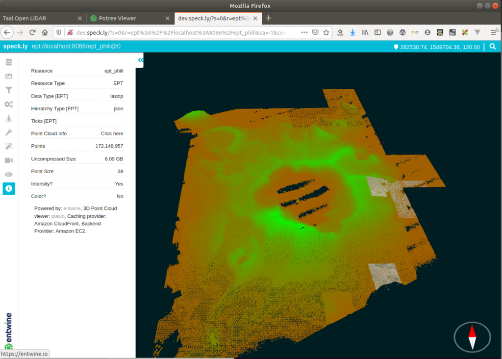
plasio about

Finding the boundary (src)
Create a JSON file named entwine.json, containing the above code, then convert from EPT to LAZ using the pdal pipeline command.
{
    "pipeline": [
        {
            "type": "readers.ept",
            "filename":"ept_phili",
            "resolution": 5
        },
        {
            "type": "writers.las",
            "compression": "true",
            "minor_version": "2",
            "dataformat_id": "0",
            "filename":"temp_data/ept_phili_to_laz.laz"
        }
    ]
}
pdal pipeline entwine.json -v 7
pdal info temp_data/ept_phili_to_laz.laz | jq .stats.bbox.native.bbox
pdal info temp_data/ept_phili_to_laz.laz -p 0(new_clouds) myuser@comp:~/phili$ pdal pipeline entwine.json -v 7
(PDAL Debug) Debugging...
(pdal pipeline readers.ept Debug) Endpoint: ept_phili/
Got EPT info
SRS: PROJCS["WGS 84 / UTM zone 51N",
GEOGCS["WGS 84",
DATUM["WGS_1984",
SPHEROID["WGS 84",6378137,298.257223563,
AUTHORITY["EPSG","7030"]],
AUTHORITY["EPSG","6326"]],
PRIMEM["Greenwich",0,
AUTHORITY["EPSG","8901"]],
UNIT["degree",0.0174532925199433,
AUTHORITY["EPSG","9122"]],
AUTHORITY["EPSG","4326"]],
PROJECTION["Transverse_Mercator"],
PARAMETER["latitude_of_origin",0],
PARAMETER["central_meridian",123],
PARAMETER["scale_factor",0.9996],
PARAMETER["false_easting",500000],
PARAMETER["false_northing",0],
UNIT["metre",1,
AUTHORITY["EPSG","9001"]],
AXIS["Easting",EAST],
AXIS["Northing",NORTH],
AUTHORITY["EPSG","32651"]]
Root resolution: 59.8594
Query resolution: 5
Actual resolution: 3.74121
Depth end: 5
Query bounds: ([-1.797693134862316e+308, 1.797693134862316e+308], [-1.797693134862316e+308, 1.797693134862316e+308], [-1.797693134862316e+308, 1.797693134862316e+308])
Threads: 4
(pdal pipeline readers.ept Debug) Registering dim X: double
(pdal pipeline readers.ept Debug) Registering dim Y: double
(pdal pipeline readers.ept Debug) Registering dim Z: double
(pdal pipeline readers.ept Debug) Registering dim Intensity: uint16_t
(pdal pipeline readers.ept Debug) Registering dim ReturnNumber: uint8_t
(pdal pipeline readers.ept Debug) Registering dim NumberOfReturns: uint8_t
(pdal pipeline readers.ept Debug) Registering dim ScanDirectionFlag: uint8_t
(pdal pipeline readers.ept Debug) Registering dim EdgeOfFlightLine: uint8_t
(pdal pipeline readers.ept Debug) Registering dim Classification: uint8_t
(pdal pipeline readers.ept Debug) Registering dim ScanAngleRank: float
(pdal pipeline readers.ept Debug) Registering dim UserData: uint8_t
(pdal pipeline readers.ept Debug) Registering dim PointSourceId: uint16_t
(pdal pipeline readers.ept Debug) Registering dim GpsTime: double
(pdal pipeline readers.ept Debug) Registering dim OriginId: uint32_t
(pdal pipeline Debug) Executing pipeline in stream mode.
(pdal pipeline readers.ept Debug) Overlap nodes: 309
(pdal pipeline readers.ept Debug) Overlap points: 8215660
(pdal pipeline readers.ept Debug) Streaming Data 1/309: 0-0-0-0
(pdal pipeline readers.ept Debug) Points : 12614
[...]
(pdal pipeline readers.ept Debug) Streaming Data 309/309: 4-14-9-7
(pdal pipeline readers.ept Debug) Points : 56730
(pdal pipeline writers.las Debug) Wrote 8215660 points to the LAS file
(new_clouds) myuser@comp:~/phili$ pdal info temp_data/ept_phili_to_laz.laz | jq .stats.bbox.native.bbox
{
"maxx": 286999.99,
"maxy": 1553999.99,
"maxz": 379.23,
"minx": 280427.84,
"miny": 1546340.11,
"minz": -139.2
}
(new_clouds) myuser@comp:~/phili$ pdal info temp_data/ept_phili_to_laz.laz -p 0
{
"filename": "temp_data/ept_phili_to_laz.laz",
"pdal_version": "2.0.1 (git-version: 6600e6)",
"points":
{
"point":
{
"Classification": 14,
"EdgeOfFlightLine": 1,
"Intensity": 1,
"NumberOfReturns": 1,
"PointId": 0,
"PointSourceId": 1010,
"ReturnNumber": 1,
"ScanAngleRank": 14,
"ScanDirectionFlag": 0,
"UserData": 0,
"X": 285540.57,
"Y": 1553975.03,
"Z": 49.87
}
}
}
(new_clouds) myuser@comp:~/phili$Get the boundary of the fitting polygon for the data as WKT or JSON.
pdal info temp_data/ept_phili_to_laz.laz --boundary(new_clouds) myuser@comp:~/phili$ pdal info temp_data/ept_phili_to_laz.laz --boundary
{
"boundary":
{
"area": 72703609.64,
"avg_pt_per_sq_unit": 28.76052946,
"avg_pt_spacing": 2.974793047,
"boundary": "POLYGON ((284777.03 1544717.6,287831.19 1547362.6,287067.65 1556620.0,277905.18 1551330.1,280959.33 1546040.1,284777.03 1544717.6))",
"boundary_json": { "type": "Polygon", "coordinates": [ [ [ 284777.030648400017526, 1544717.607343849958852 ], [ 287831.188054799975362, 1547362.585245609981939 ], [ 287067.648703199985903, 1556620.007901760051027 ], [ 277905.17648399999598, 1551330.052098240004852 ], [ 280959.333890400012024, 1546040.096294729970396 ], [ 284777.030648400017526, 1544717.607343849958852 ] ] ] },
"density": 0.1130020922,
"edge_length": 0,
"estimated_edge": 2644.977902,
"hex_offsets": "MULTIPOINT (0 0, -763.539 1322.49, 0 2644.98, 1527.08 2644.98, 2290.62 1322.49, 1527.08 0)",
"sample_size": 5000,
"threshold": 15
},
"filename": "temp_data/ept_phili_to_laz.laz",
"pdal_version": "2.0.1 (git-version: 6600e6)"
}
(new_clouds) myuser@comp:~/phili$Get a vector geometry file using pdal tindex, the “tile index” command. Then view the file in QGIS.
# simple tindex
pdal tindex create --tindex temp_data/boundary.sqlite \
    --filespec temp_data/ept_phili_to_laz.laz \
    --t_srs "EPSG:32651" \
    -f SQLite
# set edge size for output
pdal tindex create --tindex temp_data/boundary.sqlite \
    --filespec temp_data/ept_phili_to_laz.laz \
    --filters.hexbin.edge_size=10 \
    --filters.hexbin.threshold=1 \
    --t_srs "EPSG:32651" \
    -f SQLite
(new_clouds) myuser@comp:~/phili$ tree temp_data/
temp_data/
├── boundary.sqlite
├── E280N1553_LAZ_PL1.las
├── E280N1553_LAZ_PL1_WGS.laz
└── ept_phili_to_laz.laz
0 directories, 4 files
(new_clouds) myuser@comp:~/phili$
qgis tindex boundary 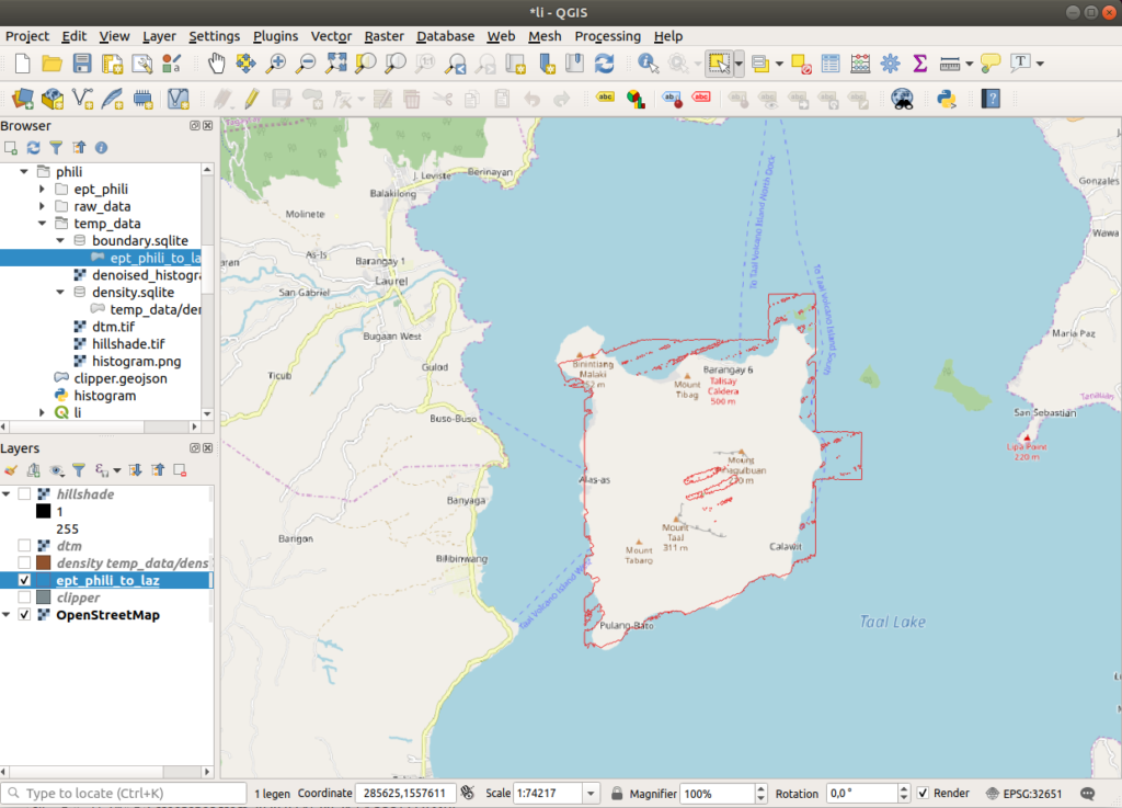
fine boundary

Or use Hexbin to output the boundary of actual points in point buffer, not just rectangular extents. Create a file named hexbin-pipeline.json and populate it with the code below, then run pdal pipeline.
[
    "temp_data/ept_phili_to_laz.laz",
    {
        "type" : "filters.hexbin"
    }
]
pdal pipeline hexbin-pipeline.json --metadata hexbin-out.json
pdal info --boundary temp_data/ept_phili_to_laz.laz(new_clouds) myuser@comp:~/phili$ tree -L 1
.
├── entwine.json
├── ept_phili
├── hexbin-out.json
├── hexbin-pipeline.json
├── raw_data
└── temp_data
3 directories, 3 files
(new_clouds) myuser@comp:~/phili$ pdal info --boundary temp_data/ept_phili_to_laz.laz
{
"boundary":
{
"area": 72703609.64,
"avg_pt_per_sq_unit": 28.76052946,
"avg_pt_spacing": 2.974793047,
"boundary": "POLYGON ((284777.03 1544717.6,287831.19 1547362.6,287067.65 1556620.0,277905.18 1551330.1,280959.33 1546040.1,284777.03 1544717.6))",
"boundary_json": { "type": "Polygon", "coordinates": [ [ [ 284777.030648400017526, 1544717.607343849958852 ], [ 287831.188054799975362, 1547362.585245609981939 ], [ 287067.648703199985903, 1556620.007901760051027 ], [ 277905.17648399999598, 1551330.052098240004852 ], [ 280959.333890400012024, 1546040.096294729970396 ], [ 284777.030648400017526, 1544717.607343849958852 ] ] ] },
"density": 0.1130020922,
"edge_length": 0,
"estimated_edge": 2644.977902,
"hex_offsets": "MULTIPOINT (0 0, -763.539 1322.49, 0 2644.98, 1527.08 2644.98, 2290.62 1322.49, 1527.08 0)",
"sample_size": 5000,
"threshold": 15
},
"filename": "temp_data/ept_phili_to_laz.laz",
"pdal_version": "2.0.1 (git-version: 6600e6)"
}
(new_clouds) myuser@comp:~/phili$Cropping
pdal translate -i temp_data/ept_phili_to_laz.laz \
   -o temp_data/ept_phili_cropped.laz \
   --readers.las.spatialreference="EPSG:32651" -f crop  \
   --filters.crop.polygon="MultiPolygon (((282066.8520627228426747 1550772.96420694049447775, 283228.65732152480632067 1551561.3320611275266856, 284763.89998494170140475 1551167.14813403389416635, 284826.13955237751360983 1550088.32896514632739127, 284348.96953536954242736 1548947.27022882294841111, 282813.72687195264734328 1548885.03066138713620603, 282046.10554024419980124 1549279.21458848076872528, 281651.92161315068369731 1550150.56853258213959634, 282066.8520627228426747 1550772.96420694049447775)))"
pdal info temp_data/ept_phili_cropped.laz --boundary
(new_clouds) myuser@comp:~/phili$ pdal translate -i temp_data/ept_phili_to_laz.laz \
> -o temp_data/ept_phili_cropped.laz \
> --readers.las.spatialreference="EPSG:32651" -f crop \
> --filters.crop.polygon="MultiPolygon (((282066.8520627228426747 1550772.96420694049447775, 283228.65732152480632067 1551561.3320611275266856, 284763.89998494170140475 1551167.14813403389416635, 284826.13955237751360983 1550088.32896514632739127, 284348.96953536954242736 1548947.27022882294841111, 282813.72687195264734328 1548885.03066138713620603, 282046.10554024419980124 1549279.21458848076872528, 281651.92161315068369731 1550150.56853258213959634, 282066.8520627228426747 1550772.96420694049447775)))"
(new_clouds) myuser@comp:~/phili$ pdal info temp_data/ept_phili_cropped.laz --boundary
{
"boundary":
{
"area": 28815222.78,
"avg_pt_per_sq_unit": 49.58609362,
"avg_pt_spacing": 4.065550131,
"boundary": "POLYGON ((284719.02 1547140.9,287236.5 1551501.3,283460.28 1553681.5,280942.8 1549321.1,284719.02 1547140.9))",
"boundary_json": { "type": "Polygon", "coordinates": [ [ [ 284719.019983169971965, 1547140.906790179898962 ], [ 287236.499949509976432, 1551501.310000000055879 ], [ 283460.28000000002794, 1553681.511604910017923 ], [ 280942.800033660023473, 1549321.108395090093836 ], [ 284719.019983169971965, 1547140.906790179898962 ] ] ] },
"density": 0.06050083365,
"edge_length": 0,
"estimated_edge": 2180.201605,
"hex_offsets": "MULTIPOINT (0 0, -629.37 1090.1, 0 2180.2, 1258.74 2180.2, 1888.11 1090.1, 1258.74 0)",
"sample_size": 5000,
"threshold": 15
},
"filename": "temp_data/ept_phili_cropped.laz",
"pdal_version": "2.0.1 (git-version: 6600e6)"
}
(new_clouds) myuser@comp:~/phili$Clipping data with polygons (src)
{
    "pipeline": [
        "temp_data/ept_phili_to_laz.laz",
        {
            "column": "CLS",
            "datasource": "clipper.geojson",
            "dimension": "Classification",
            "type": "filters.overlay"
        },
        {
            "limits": "Classification[6:6]",
            "type": "filters.range"
        },
        "temp_data/ept_phili_clipped.laz"
    ]
}
pdal pipeline clipping.json --nostreamColorizing points with imagery (src)
TODO
Removing noise (src)
Use PDAL to remove unwanted noise. Create a file named denoise.json and populate it with the following code, then run pdal pipeline.
{
    "pipeline": [
        "temp_data/ept_phili_to_laz.laz",
        {
            "type": "filters.outlier",
            "method": "statistical",
            "multiplier": 3,
            "mean_k": 8
        },
        {
            "type": "filters.range",
            "limits": "Classification![7:7],Z[-100:3000]"
        },
        {
            "type": "writers.las",
            "compression": "true",
            "minor_version": "2",
            "dataformat_id": "0",
            "filename":"temp_data/clean.laz"
        }
    ]
}
pdal pipeline denoise.json(new_clouds) myuser@comp:~/phili$ pdal pipeline denoise.json
(new_clouds) myuser@comp:~/phili$ tree temp_data/
temp_data/
├── boundary.sqlite
├── clean.laz
├── E280N1553_LAZ_PL1.las
├── E280N1553_LAZ_PL1_WGS.laz
└── ept_phili_to_laz.laz
0 directories, 5 files
(new_clouds) myuser@comp:~/phili$ pdal info --boundary temp_data/clean.laz
{
"boundary":
{
"area": 81355357.53,
"avg_pt_per_sq_unit": 29.95675523,
"avg_pt_spacing": 3.159997638,
"boundary": "POLYGON ((284609.97 1544906.0,289844.42 1548791.5,286853.31 1556562.7,277879.96 1551381.9,280871.08 1546201.2,284609.97 1544906.0))",
"boundary_json": { "type": "Polygon", "coordinates": [ [ [ 284609.971245159977116, 1544905.9744242799934 ], [ 289844.422529059986118, 1548791.546813880093396 ], [ 286853.307509689999279, 1556562.691593060037121 ], [ 277879.962451570027042, 1551381.928406940074638 ], [ 280871.077470940013882, 1546201.165220810100436 ], [ 284609.971245159977116, 1544905.9744242799934 ] ] ] },
"density": 0.1001443574,
"edge_length": 0,
"estimated_edge": 2590.381593,
"hex_offsets": "MULTIPOINT (0 0, -747.779 1295.19, 0 2590.38, 1495.56 2590.38, 2243.34 1295.19, 1495.56 0)",
"sample_size": 5000,
"threshold": 15
},
"filename": "temp_data/clean.laz",
"pdal_version": "2.0.1 (git-version: 6600e6)"
}Visualizing acquisition density (src)
Generate a density surface to summarize acquisition quality, and visualize it in QGIS, applying a gradient color ramp and using the count attribute.
pdal density temp_data/ept_phili_to_laz.laz  \
    -o temp_data/density.sqlite \
    -f SQLite
Acquisition density
Thinning (src)
Subsample or thin point cloud data, to accelerate processing (less data), normalize point density, or ease visualization.
pdal translate temp_data/ept_phili_to_laz.laz \
    temp_data/thin.laz \
    sample --filters.sample.radius=20
(new_clouds) myuser@comp:~/phili$ pdal translate temp_data/ept_phili_to_laz.laz \
> temp_data/thin.laz \
> sample --filters.sample.radius=20
(new_clouds) myuser@comp:~/phili$ tree temp_data/
temp_data/
├── boundary.sqlite
├── clean.laz
├── density.sqlite
├── E280N1553_LAZ_PL1.las
├── E280N1553_LAZ_PL1_WGS.laz
├── ept_phili_to_laz.laz
└── thin.laz
0 directories, 7 files
(new_clouds) myuser@comp:~/phili$Identifying ground (src)
You can classify ground returns using the Simple Morphological Filter (SMRF) technique.
pdal translate temp_data/ept_phili_to_laz.laz \
    -o temp_data/ground.laz \
    smrf \
    -v 4
To aquire a more accurate representation of the ground returns, you can remove the non-ground data to just view the ground data, then use the translate command to stack the filters.outlier and filters.smrf.
pdal translate \
    temp_data/ept_phili_to_laz.laz \
    -o temp_data/ground.laz \
    smrf range \
    --filters.range.limits="Classification[2:2]" \
    -v 4
Let’s run only the next command, to spare some time, usually this process lasts longer.
pdal translate temp_data/ept_phili_to_laz.laz \
    -o temp_data/denoised_ground.laz \
    outlier smrf range  \
    --filters.outlier.method="statistical" \
    --filters.outlier.mean_k=8 --filters.outlier.multiplier=3.0 \
    --filters.smrf.ignore="Classification[7:7]"  \
    --filters.range.limits="Classification[2:2]" \
    --writers.las.compression=true \
    --verbose 4
(new_clouds) myuser@comp:~/phili$ pdal translate temp_data/ept_phili_to_laz.laz \
> -o temp_data/denoised_ground.laz \
> outlier smrf range \
> --filters.outlier.method="statistical" \
> --filters.outlier.mean_k=8 --filters.outlier.multiplier=3.0 \
> --filters.smrf.ignore="Classification[7:7]" \
> --filters.range.limits="Classification[2:2]" \
> --writers.las.compression=true \
> --verbose 4
(PDAL Debug) Debugging...
(pdal translate Debug) Executing pipeline in standard mode.
(pdal translate filters.smrf Debug) progressiveFilter: radius = 1 50115212 ground 141946 non-ground (0.28%)
(pdal translate filters.smrf Debug) progressiveFilter: radius = 1 41616570 ground 8640588 non-ground (17.19%)
(pdal translate filters.smrf Debug) progressiveFilter: radius = 2 37966057 ground 12291101 non-ground (24.46%)
(pdal translate filters.smrf Debug) progressiveFilter: radius = 3 35656784 ground 14600374 non-ground (29.05%)
(pdal translate filters.smrf Debug) progressiveFilter: radius = 4 34547497 ground 15709661 non-ground (31.26%)
(pdal translate filters.smrf Debug) progressiveFilter: radius = 5 34005642 ground 16251516 non-ground (32.34%)
(pdal translate filters.smrf Debug) progressiveFilter: radius = 6 33701727 ground 16555431 non-ground (32.94%)
(pdal translate filters.smrf Debug) progressiveFilter: radius = 7 33509838 ground 16747320 non-ground (33.32%)
(pdal translate filters.smrf Debug) progressiveFilter: radius = 8 33374281 ground 16882877 non-ground (33.59%)
(pdal translate filters.smrf Debug) progressiveFilter: radius = 9 33279882 ground 16977276 non-ground (33.78%)
(pdal translate filters.smrf Debug) progressiveFilter: radius = 10 33212965 ground 17044193 non-ground (33.91%)
(pdal translate filters.smrf Debug) progressiveFilter: radius = 11 33162742 ground 17094416 non-ground (34.01%)
(pdal translate filters.smrf Debug) progressiveFilter: radius = 12 33128547 ground 17128611 non-ground (34.08%)
(pdal translate filters.smrf Debug) progressiveFilter: radius = 13 33105320 ground 17151838 non-ground (34.13%)
(pdal translate filters.smrf Debug) progressiveFilter: radius = 14 33089489 ground 17167669 non-ground (34.16%)
(pdal translate filters.smrf Debug) progressiveFilter: radius = 15 33080329 ground 17176829 non-ground (34.18%)
(pdal translate filters.smrf Debug) progressiveFilter: radius = 16 33074261 ground 17182897 non-ground (34.19%)
(pdal translate filters.smrf Debug) progressiveFilter: radius = 17 33070615 ground 17186543 non-ground (34.20%)
(pdal translate filters.smrf Debug) progressiveFilter: radius = 18 33068555 ground 17188603 non-ground (34.20%)
(pdal translate writers.las Debug) Wrote 3776158 points to the LAS file
(new_clouds) myuser@comp:~/phili$Generating a DTM (src)
Generate an elevation model surface using the output from above. Create a file named dtm.json and populate it with the code below, then run pdal pipeline.
{
    "pipeline": [
        "temp_data/denoised_ground.laz",
        {
            "filename":"temp_data/dtm.tif",
            "gdaldriver":"GTiff",
            "output_type":"all",
            "resolution":"2.0",
            "type": "writers.gdal"
        }
    ]
}
pdal pipeline dtm.json(new_clouds) myuser@comp:~/phili$ pdal pipeline dtm.json
(new_clouds) myuser@comp:~/phili$ tree temp_data/
temp_data/
├── boundary.sqlite
├── clean.laz
├── denoised_ground.laz
├── density.sqlite
├── dtm.tif
├── E280N1553_LAZ_PL1.las
├── E280N1553_LAZ_PL1_WGS.laz
├── ept_phili_to_laz.laz
├── ground.laz
└── thin.laz
0 directories, 10 files
(new_clouds) myuser@comp:~/phili$
DTM
Generate a Hillshade from the DTM (Digital Terrain Model).
gdaldem hillshade temp_data/dtm.tif \
    temp_data/hillshade.tif \
    -z 1.0 -s 1.0 -az 315.0 -alt 45.0 \
    -of GTiff
(new_clouds) myuser@comp:~/phili$ gdaldem hillshade temp_data/dtm.tif \
> temp_data/hillshade.tif \
> -z 1.0 -s 1.0 -az 315.0 -alt 45.0 \
> -of GTiff
0...10...20...30...40...50...60...70...80...90...100 - done.
(new_clouds) myuser@comp:~/phili$ tree temp_data/
temp_data/
├── boundary.sqlite
├── clean.laz
├── denoised_ground.laz
├── density.sqlite
├── dtm.tif
├── E280N1553_LAZ_PL1.las
├── E280N1553_LAZ_PL1_WGS.laz
├── ept_phili_to_laz.laz
├── ground.laz
├── hillshade.tif
└── thin.laz
0 directories, 11 files
(new_clouds) myuser@comp:~/phili$
hillshade
Creating surface meshes (src)
TODO
Rasterizing Attributes (src)
Generate a raster surface using a fully classified point cloud. Create a file named classification.json and populate it with the below code, then run pdal pipeline.
{
    "pipeline":[
        {
            "type":"readers.ept",
            "filename":"ept_phili",
            "resolution": 5
        },
        {
            "type":"writers.gdal",
            "filename":"temp_data/phili-classification.tif",
            "dimension":"Classification",
            "data_type":"uint16_t",
            "output_type":"mean",
            "resolution": 5
        }
    ]
}
pdal pipeline classification.json -v 3(new_clouds) myuser@comp:~/phili$ pdal pipeline classification.json -v 3
(PDAL Debug) Debugging...
(pdal pipeline readers.ept Debug) Endpoint: ept_phili/
Got EPT info
SRS: PROJCS["WGS 84 / UTM zone 51N",
GEOGCS["WGS 84",
DATUM["WGS_1984",
SPHEROID["WGS 84",6378137,298.257223563,
AUTHORITY["EPSG","7030"]],
AUTHORITY["EPSG","6326"]],
PRIMEM["Greenwich",0,
AUTHORITY["EPSG","8901"]],
UNIT["degree",0.0174532925199433,
AUTHORITY["EPSG","9122"]],
AUTHORITY["EPSG","4326"]],
PROJECTION["Transverse_Mercator"],
PARAMETER["latitude_of_origin",0],
PARAMETER["central_meridian",123],
PARAMETER["scale_factor",0.9996],
PARAMETER["false_easting",500000],
PARAMETER["false_northing",0],
UNIT["metre",1,
AUTHORITY["EPSG","9001"]],
AXIS["Easting",EAST],
AXIS["Northing",NORTH],
AUTHORITY["EPSG","32651"]]
Root resolution: 59.8594
Query resolution: 5
Actual resolution: 3.74121
Depth end: 5
Query bounds: ([-1.797693134862316e+308, 1.797693134862316e+308], [-1.797693134862316e+308, 1.797693134862316e+308], [-1.797693134862316e+308, 1.797693134862316e+308])
Threads: 4
(pdal pipeline readers.ept Debug) Registering dim X: double
(pdal pipeline readers.ept Debug) Registering dim Y: double
(pdal pipeline readers.ept Debug) Registering dim Z: double
(pdal pipeline readers.ept Debug) Registering dim Intensity: uint16_t
(pdal pipeline readers.ept Debug) Registering dim ReturnNumber: uint8_t
(pdal pipeline readers.ept Debug) Registering dim NumberOfReturns: uint8_t
(pdal pipeline readers.ept Debug) Registering dim ScanDirectionFlag: uint8_t
(pdal pipeline readers.ept Debug) Registering dim EdgeOfFlightLine: uint8_t
(pdal pipeline readers.ept Debug) Registering dim Classification: uint8_t
(pdal pipeline readers.ept Debug) Registering dim ScanAngleRank: float
(pdal pipeline readers.ept Debug) Registering dim UserData: uint8_t
(pdal pipeline readers.ept Debug) Registering dim PointSourceId: uint16_t
(pdal pipeline readers.ept Debug) Registering dim GpsTime: double
(pdal pipeline readers.ept Debug) Registering dim OriginId: uint32_t
(pdal pipeline Debug) Executing pipeline in stream mode.
(pdal pipeline readers.ept Debug) Overlap nodes: 309
(pdal pipeline readers.ept Debug) Overlap points: 8215660
(pdal pipeline readers.ept Debug) Streaming Data 1/309: 0-0-0-0
(pdal pipeline readers.ept Debug) Points : 12614
(pdal pipeline readers.ept Debug) Streaming Data 2/309: 1-0-0-0
(pdal pipeline readers.ept Debug) Points : 10146
(pdal pipeline readers.ept Debug) Streaming Data 3/309: 1-0-0-1
[...]
(pdal pipeline readers.ept Debug) Points : 38612
(pdal pipeline readers.ept Debug) Streaming Data 309/309: 4-14-9-7
(pdal pipeline readers.ept Debug) Points : 56730
(new_clouds) myuser@comp:~/phili$(new_clouds) myuser@comp:~/phili$ tree temp_data/
temp_data/
├── boundary.sqlite
├── clean.laz
├── clipper.geojson.tmp
├── denoised_ground.laz
├── denoised_histogram.png
├── density.sqlite
├── dtm.tif
├── E280N1553_LAZ_PL1.las
├── E280N1553_LAZ_PL1_WGS.laz
├── ept_phili_clipped.laz
├── ept_phili_cropped.laz
├── ept_phili_to_laz.laz
├── ground.laz
├── hillshade.tif
├── histogram.png
├── phili-classification.tif
└── thin.laz
0 directories, 17 files
(new_clouds) myuser@comp:~/phili$
rasterize
Then create a file named colours.txt and enter the code below, that gdaldem can consume to apply colors to the data, and QGIS can use as color map.
# QGIS Generated Color Map Export File
2 139 51 38 255 Ground
3 143 201 157 255 Low Veg
4 5 159 43 255 Med Veg
5 47 250 11 255 High Veg
6 209 151 25 255 Building
7 232 41 7 255 Low Point
8 197 0 204 255 reserved
9 26 44 240 255 Water
10 165 160 173 255 Rail
11 81 87 81 255 Road
12 203 210 73 255 Reserved
13 209 228 214 255 Wire - Guard (Shield)
14 160 168 231 255 Wire - Conductor (Phase)
15 220 213 164 255 Transmission Tower
16 214 211 143 255 Wire-Structure Connector (Insulator)
17 151 98 203 255 Bridge Deck
18 236 49 74 255 High Noise
19 185 103 45 255 Reserved
21 58 55 9 255 255 Reserved
22 76 46 58 255 255 Reserved
23 20 76 38 255 255 Reserved
26 78 92 32 255 255 Reserved
gdaldem color-relief temp_data/phili-classification.tif colours.txt temp_data/classified-color.png -of PNG(new_clouds) myuser@comp:~/phili$ gdaldem color-relief temp_data/phili-classification.tif colours.txt temp_data/classified-color.png -of PNG
0...10...20...30...40...50...60...70...80...90...100 - done.
(new_clouds) myuser@comp:~/phili$
classified color
Then generate a relative intensity image.
pdal pipeline classification.json \
    --writers.gdal.dimension="Intensity" \
    --writers.gdal.data_type="float" \
    --writers.gdal.filename="temp_data/intensity.tif" \
    -v 3
pdal pipeline classification.json \
> --writers.gdal.dimension="Intensity" \
> --writers.gdal.data_type="float" \
> --writers.gdal.filename="temp_data/intensity.tif" \
> -v 3
(PDAL Debug) Debugging...
(pdal pipeline readers.ept Debug) Endpoint: ept_phili/
Got EPT info
SRS: PROJCS["WGS 84 / UTM zone 51N",
GEOGCS["WGS 84",
DATUM["WGS_1984",
SPHEROID["WGS 84",6378137,298.257223563,
AUTHORITY["EPSG","7030"]],
AUTHORITY["EPSG","6326"]],
PRIMEM["Greenwich",0,
AUTHORITY["EPSG","8901"]],
UNIT["degree",0.0174532925199433,
AUTHORITY["EPSG","9122"]],
AUTHORITY["EPSG","4326"]],
PROJECTION["Transverse_Mercator"],
PARAMETER["latitude_of_origin",0],
PARAMETER["central_meridian",123],
PARAMETER["scale_factor",0.9996],
PARAMETER["false_easting",500000],
PARAMETER["false_northing",0],
UNIT["metre",1,
AUTHORITY["EPSG","9001"]],
AXIS["Easting",EAST],
AXIS["Northing",NORTH],
AUTHORITY["EPSG","32651"]]
Root resolution: 59.8594
Query resolution: 5
Actual resolution: 3.74121
Depth end: 5
Query bounds: ([-1.797693134862316e+308, 1.797693134862316e+308], [-1.797693134862316e+308, 1.797693134862316e+308], [-1.797693134862316e+308, 1.797693134862316e+308])
Threads: 4
(pdal pipeline readers.ept Debug) Registering dim X: double
(pdal pipeline readers.ept Debug) Registering dim Y: double
(pdal pipeline readers.ept Debug) Registering dim Z: double
(pdal pipeline readers.ept Debug) Registering dim Intensity: uint16_t
(pdal pipeline readers.ept Debug) Registering dim ReturnNumber: uint8_t
(pdal pipeline readers.ept Debug) Registering dim NumberOfReturns: uint8_t
(pdal pipeline readers.ept Debug) Registering dim ScanDirectionFlag: uint8_t
(pdal pipeline readers.ept Debug) Registering dim EdgeOfFlightLine: uint8_t
(pdal pipeline readers.ept Debug) Registering dim Classification: uint8_t
(pdal pipeline readers.ept Debug) Registering dim ScanAngleRank: float
(pdal pipeline readers.ept Debug) Registering dim UserData: uint8_t
(pdal pipeline readers.ept Debug) Registering dim PointSourceId: uint16_t
(pdal pipeline readers.ept Debug) Registering dim GpsTime: double
(pdal pipeline readers.ept Debug) Registering dim OriginId: uint32_t
(pdal pipeline Debug) Executing pipeline in stream mode.
(pdal pipeline readers.ept Debug) Overlap nodes: 309
(pdal pipeline readers.ept Debug) Overlap points: 8215660
(pdal pipeline readers.ept Debug) Streaming Data 1/309: 0-0-0-0
(pdal pipeline readers.ept Debug) Points : 12614
(pdal pipeline readers.ept Debug) Streaming Data 2/309: 1-0-0-0
(pdal pipeline readers.ept Debug) Points : 10146
(pdal pipeline readers.ept Debug) Streaming Data 3/309: 1-0-0-1
(pdal pipeline readers.ept Debug) Points : 33239
(pdal pipeline readers.ept Debug) Streaming Data 4/309: 1-0-1-0
(pdal pipeline readers.ept Debug) Points : 9649
(pdal pipeline readers.ept Debug) Streaming Data 5/309: 1-0-1-1
[...]
(pdal pipeline readers.ept Debug) Points : 38612
(pdal pipeline readers.ept Debug) Streaming Data 309/309: 4-14-9-7
(pdal pipeline readers.ept Debug) Points : 56730
(new_clouds) myuser@comp:~/phili$gdal_translate temp_data/intensity.tif temp_data/intensity.png -of PNG(new_clouds) myuser@comp:~/phili$ gdal_translate temp_data/intensity.tif temp_data/intensity.png -of PNG
Input file size is 1315, 1532
Warning 6: PNG driver doesn't support data type Float32. Only eight bit (Byte) and sixteen bit (UInt16) bands supported. Defaulting to Byte
0...10...20...30...40...50...60...70...80...90...100 - done.
(new_clouds) myuser@comp:~/phili$
intensity original 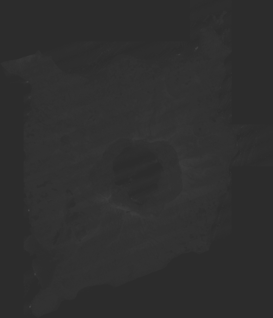
intensity increased brightness


Plotting a histogram using Python (src)
{
    "pipeline": [
        {
            "filename": "temp_data/ept_phili_to_laz.laz"
        },
        {
            "type": "filters.python",
            "function": "make_plot",
            "module": "anything",
            "pdalargs": "{\"filename\":\"temp_data/histogram.png\"}",
            "script": "histogram.py"
        },
        {
            "type": "writers.null"
        }
    ]
}
# import numpy
import numpy as np
# import matplotlib stuff and make sure to use the
# AGG renderer.
import matplotlib
matplotlib.use('Agg')
import matplotlib.pyplot as plt
import matplotlib.mlab as mlab
# This only works for Python 3. Use
# StringIO for Python 2.
from io import BytesIO
# The make_plot function will do all of our work. The
# filters.programmable filter expects a function name in the
# module that has at least two arguments -- "ins" which
# are numpy arrays for each dimension, and the "outs" which
# the script can alter/set/adjust to have them updated for
# further processing.
def make_plot(ins, outs):
# figure position and row will increment
figure_position = 1
row = 1
fig = plt.figure(figure_position, figsize=(6, 8.5), dpi=300)
for key in ins:
dimension = ins[key]
ax = fig.add_subplot(len(ins.keys()), 1, row)
# histogram the current dimension with 30 bins
n, bins, patches = ax.hist( dimension, 30,
facecolor='grey',
alpha=0.75,
align='mid',
histtype='stepfilled',
linewidth=None)
# Set plot particulars
ax.set_ylabel(key, size=10, rotation='horizontal')
ax.get_xaxis().set_visible(False)
ax.set_yticklabels('')
ax.set_yticks((),)
ax.set_xlim(min(dimension), max(dimension))
ax.set_ylim(min(n), max(n))
# increment plot position
row = row + 1
figure_position = figure_position + 1
# We will save the PNG bytes to a BytesIO instance
# and the nwrite that to a file.
output = BytesIO()
plt.savefig(output,format="PNG")
# a module global variable, called 'pdalargs' is available
# to filters.programmable and filters.predicate modules that contains
# a dictionary of arguments that can be explicitly passed into
# the module by the user. We passed in a filename arg in our `pdal pipeline` call
if 'filename' in pdalargs:
filename = pdalargs['filename']
else:
filename = 'histogram.png'
# open up the filename and write out the
# bytes of the PNG stored in the BytesIO instance
o = open(filename, 'wb')
o.write(output.getvalue())
o.close()
# filters.programmable scripts need to
# return True to tell the filter it was successful.
return Truepython -m pip install -U matplotlib==3.2.0rc1
pdal pipeline histogram.json(new_clouds) myuser@comp:~/phili$ pdal pipeline histogram.json
anything:46: UserWarning: Attempting to set identical left == right == 0 results in singular transformations; automatically expanding.
(new_clouds) myuser@comp:~/phili$
Python histogram for laz file
Batch Processing (src)
# Create directory unless exists
mkdir -pv gtiles
# List files in Windows dos and iterate them
# use verbose to view logs
for %f in (*.*) do pdal pipeline denoise_ground.json ^
   --readers.las.filename=%f ^
   --writers.las.filename=../gtiles/%f
   --verbose 4

# Create directory unless exists
mkdir -pv denoised_grnd
# List files in Linux shell and iterate them
ls laz_tiles/*.laz | \
parallel -I{} pdal pipeline denoise_ground.json \
    --readers.las.filename={} \
    --writers.las.filename=denoised_grnd/denoised_grnd{/.}.laz \
    --verbose 4
What’s next?
☑️ Repeat the steps for Yosemite Valley
☑️ Then try LasTools, too
☑️ And, of course, the 3D in Blender. 😀
PS: The people from Taal Open LiDAR Data gave acces in the meantime to the Potree 3D visualization, if you like you can admire it here.
Below, I leave you a Potree mix from my personal computer.
